CS224N W5. Self attention and Transformer

All contents is arranged from CS224N contents. Please see the details to the CS224N!

1. Issue with recurrent models

$\checkmark$ Linear interaction distance

RNNs take O(sequence length) steps for distant word pairs to interact.

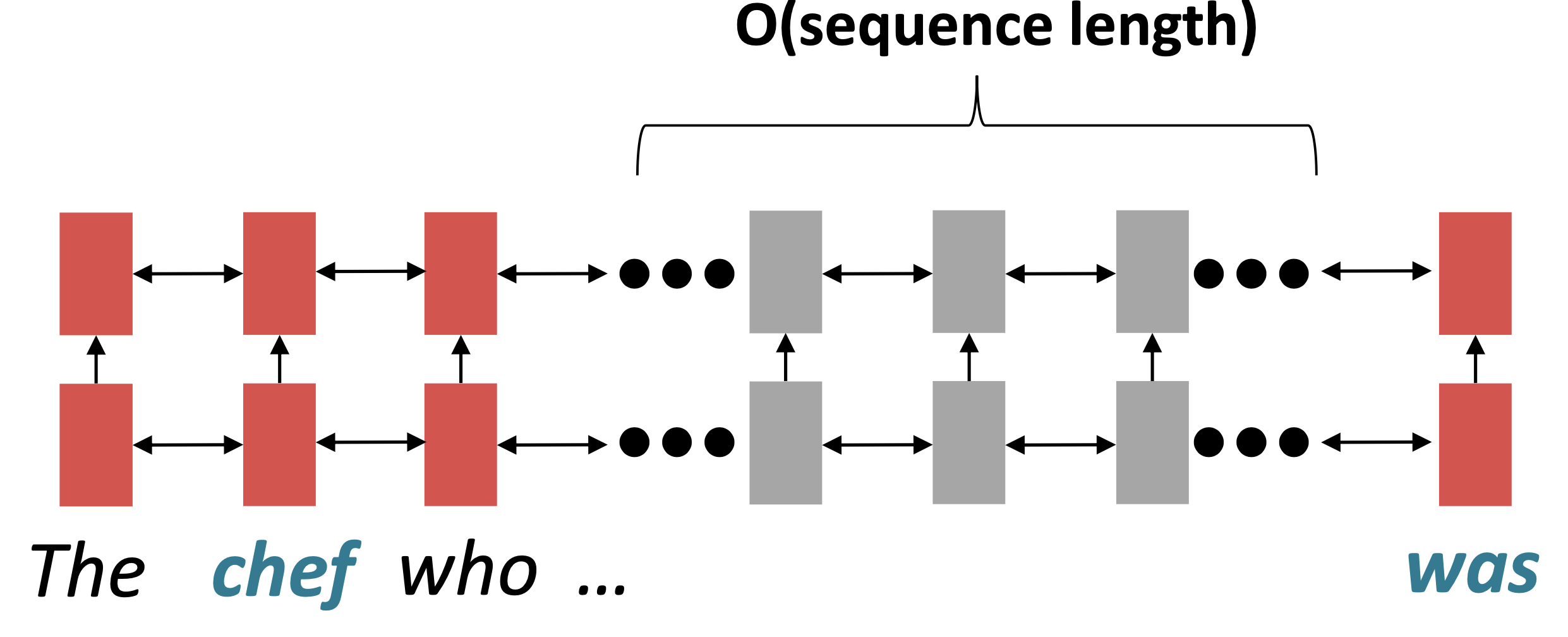
Reference. Stanford CS224n, 2021, Before word 'was', Information of chef has gone through O(sequence length) many layers!

It’s Hard to learn long-distance dependencies because of gradient problems. And linear order of words is “baked in”; we already know linear order isn’t the right way to think about sentences.

$\checkmark$ Lack of parallelizability

2. If not recurrence, then what?

2.1 Word windows, also known as 1D convolution

Word window models aggregate local contexts

Reference. Stanford CS224n, 2021, Number of unparallelizable operations does not increase sequence length

• Long-distance dependencies: Stacking word window layers allows interaction between farther words
• Maximum Interaction distance = sequence length / window size, but if sequence are too long, you’ll just ignore long-distance context

Reference. Stanford CS224n, 2021

2.2 Attention

• Attention treats each word’s representation as a query to access and incorporate information from a set of values.
• Number of unparallelizable operations does not increase sequence length.
• Maximum interaction distance: O(1), since all words interact at every layer.

Reference. Stanford CS224n, 2021

3. Self-Attention

• Reference. https://jalammar.github.io/illustrated-transformer/

3.1 Overview

1. Attention operates on queries, keys, and values.

   \[\begin{aligned} &\text{Queries, } q_1, q_2, \dots,q_T, q_i \in \mathbb{R}^d \\ &\text{Keys, } k_1, k_2, \dots,k_T, k_i \in \mathbb{R}^d \\ &\text{Values, } v_1, v_2, \dots,v_T, v_i \in \mathbb{R}^d \\ \end{aligned}\]

2. In self-attention, the queries, keys, and values are drawn from the same source.

   For example, if the output of the previous layer is $𝑥_1, … , 𝑥_𝑇$, (one vec per word) we could let $𝑣_𝑖 = 𝑘_𝑖 = 𝑞_𝑖 = 𝑥_𝑖$ (that is, use the same vectors for all of them!).

   In transformer model, it defines,

   \[𝑣_𝑖 = Vx_i,\ 𝑘_𝑖 = Kx_i,\ 𝑞_𝑖 = Qx_i,\ K,\ Q,\ V \in \mathbb{R}^{d\times d}\]

   And we use V and K in encoder for decoder

3. The (dot product) self-attention operation is as follows:

   

   Reference. Stanford CS224n, 2021

4. NLP building Block

   

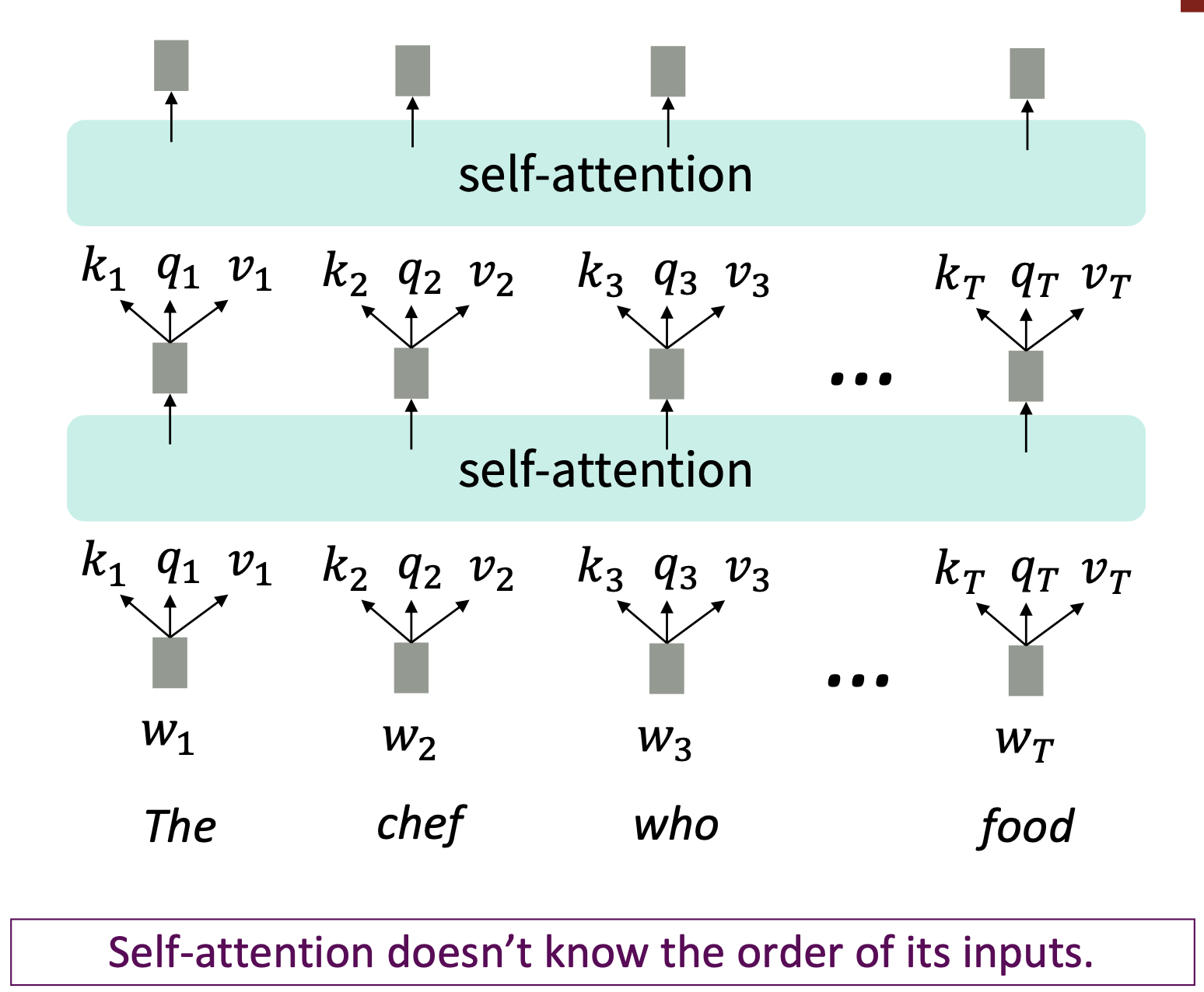
   Reference. Stanford CS224n, 2021, Self-attention is an operation on sets. It has no inherent notion of order.

   Self-attention is an operation on sets. It has no inherent notion of order.

3.2 Barriers and solutions for Self-Attention as a building block

$\checkmark$ 1. Doesn’t have an inherent notion for order → Add position representations to the inputs

Since self-attention doesn’t build in order information, we need to encode the order of the sentence in our keys, queries, and values. Consider representing each sequence index as a vector

Easy to incorporate this info into our self-attention block: just add the 𝑝𝑖 to our inputs. Let $\tilde{v_i},\ \tilde{k_i},\ \tilde{q_i}$ be our old values, keys, and queries.

In deep self-attention networks, we do this at the first layer! You could concatenate them as well, but people mostly just add…

Method 1 Sinusoidal position representations. 

• concatenate sinusoidal functions of varying periods:

  \[p_i = \begin{bmatrix} sin(i/10000^{2*1/d})\\ cos(i/10000^{2*1/d})\\ \vdots\\ sin(i/10000^{2*\frac{d}{2}/d})\\ cos(i/10000^{2*\frac{d}{2}/d})\\ \end{bmatrix}\]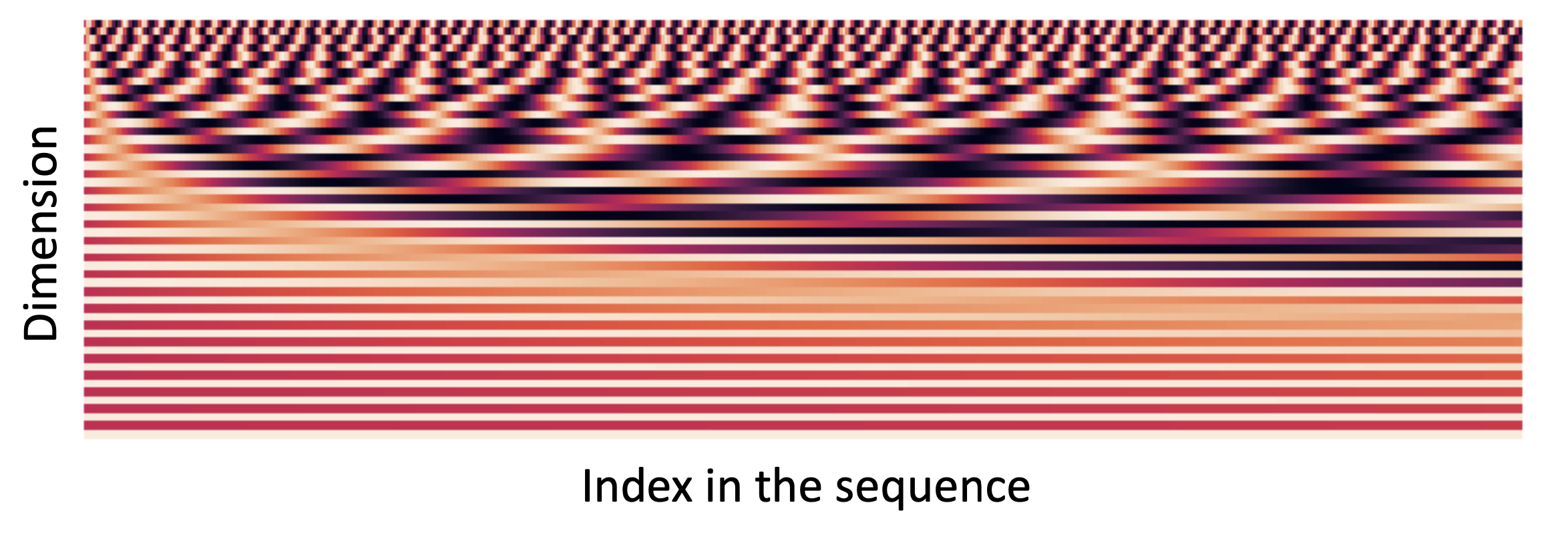

  

  Reference. Stanford CS224n, 2021

• Pros
  • Periodicity indicates that maybe “absolute position” isn’t as important
  • Maybe can extrapolate to longer sequences as periods restart!
• Cons
  • Not learnable
  • The extrapolation doesn’t really work!

Method 2 Position representation vectors learned from scratch.

• Learned absolute position representations: Let all $p_i$ be learnable parameters! Learn a matrix $𝑝 \in \mathbb{R}^{𝑑\times 𝑇}$, and let each $p_i$ be a column of that matrix
• Pros: Flexibility, each position gets to be learned to fit the data
• Cons: Definitely can’t extrapolate to indices outside 1, … , 𝑇.

Most systems use this. Sometimes people try more flexible representations of position:

• Relative linear position attention [Shaw et al., 2018]
• Dependency syntax-based position [Wang et al., 2019]

$\checkmark$ 2. No nonlinearities for deep learning. It’s all just weighted averages → adding the same feedforward network to each self-attention output

• Adding Nonlinearities in self-attention

  Note that there are no elementwise nonlinearities in self-attention; stacking more self-attention layers just re-averages value vectors.

  Add a feed-forward network to post-process each output vector($W_2, b_2$ in below equation)

  \[\begin{aligned} m_i &= \text{MLP}(\text{output}_i)\\ &= W_2 * \text{ReLU}(W_1 \times \text{output}_i + b_1)+b_2 \end{aligned}\]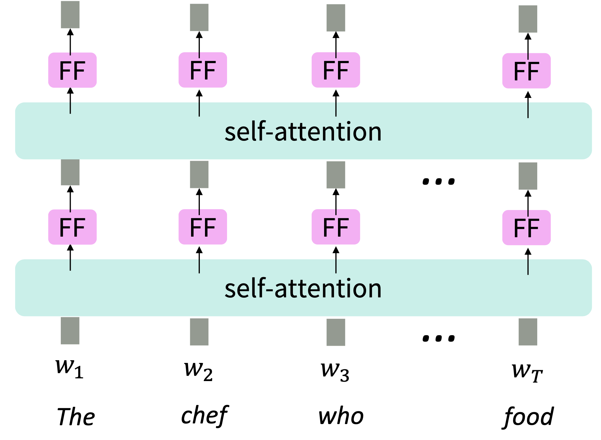

  

  Reference. Stanford CS224n, 2021, Intuition: the FF network processes the result of attention

$\checkmark$ 3. Need to ensure we don’t “look at the future” when predicting a sequence → Mask out the future by artificially setting attention weights to 0

To use self-attention in decoders, we need to ensure we can’t peek at the future. To enable parallelization, we mask out attention to future words by setting attention scores to −∞.

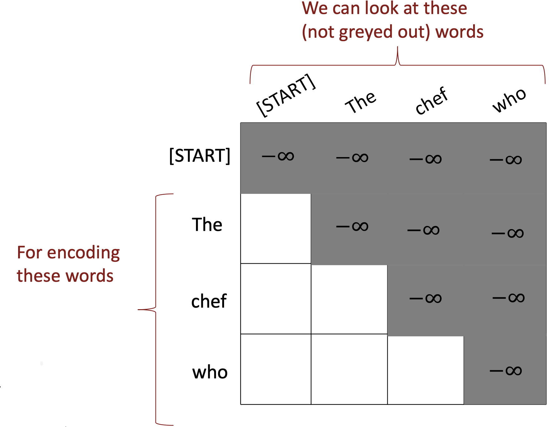
Reference. Stanford CS224n, 2021, Intuition: the FF network processes the result of attention

4. Transformer model

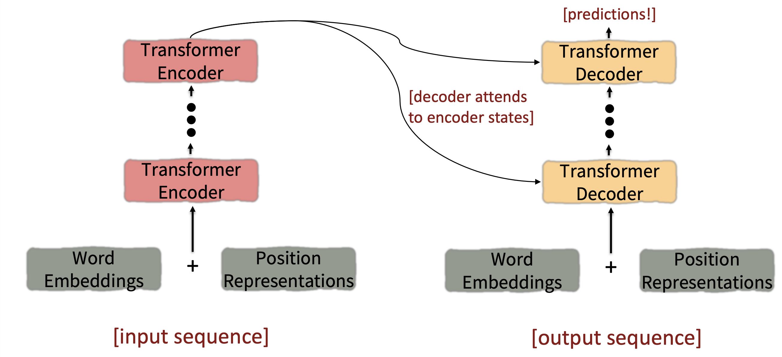
Reference. Stanford CS224n, 2021, The Transformer Encoder-Decoder [Vaswani et al., 2017]

4.1 Transformer Encoder

$\checkmark$ Key-query-value attention: How do we get the 𝑘, 𝑞, 𝑣 vectors from a single word embedding?

• We saw that self-attention is when keys, queries, and values come from the same source. The Transformer does this in a particular way:

  \[\text{Let }𝑥_1, \dots , 𝑥_𝑇\text{ be input vectors to the Transformer encoder}; 𝑥_i \in \mathbb{R}^𝑑\]

• Then keys, queries, values are:

  \[\begin{aligned} &k_i = Kx_i\text{, where } K \in \mathbb{R}^{d\times d}\text{ is the key matrix}\\ &q_i = Qx_i\text{, where } Q \in \mathbb{R}^{d\times d}\text{ is the query matrix}\\ &v_i = Vx_i\text{, where } V \in \mathbb{R}^{d\times d}\text{ is the value matrix}\\ \end{aligned}\]
• These matrices allow different aspects of the 𝑥 vectors to be used/emphasized in each of the three roles.
• Let’s look at how key-query-value attention is computed, in matrices.
  • Let $𝑋 = [𝑥_1; … ; 𝑥_𝑇] \in \mathbb{R}^{𝑇\times 𝑑}$ be the concatenation of input vectors.
  • First, note that $𝑋𝐾 \in \mathbb{R}^{𝑇\times 𝑑}, 𝑋𝑄 \in \mathbb{R}^{𝑇\times 𝑑}, 𝑋𝑉 \in \mathbb{R}^{𝑇\times 𝑑}.$
  • The output is defined as $output = softmax(𝑋𝑄(𝑋𝐾)^⊤)\times 𝑋𝑉$

  

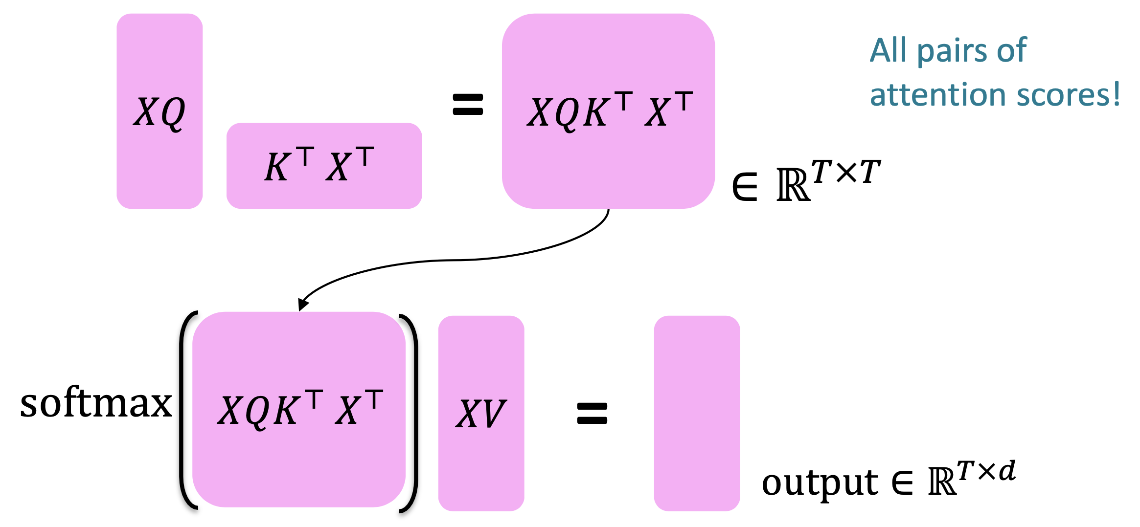
  Reference. Stanford CS224n, 2021

  First, take the query-key dot products in one matrix multiplication: $𝑋𝑄(𝑋𝐾)^⊤$. Next, softmax, and compute the weighted average with another matrix multiplication.

$\checkmark$ Multi-headed attention: Attend to multiple places in a single layer!

• What if we want to look in multiple places in the sentence at once?
  • For word i, self-attention “looks” where $𝑥_i^⊤𝑄^⊤𝐾𝑥_j$  is high, but maybe we want to focus on different j for different reasons?
• We’ll define multiple attention “heads” through multiple Q,K,V matrices

• Let, $Q_{\ell}, K_{\ell}, V_{\ell} \in \mathbb{R}^{d \times \frac{d}{h}}$, where h is the number of attention heads, and $\ell$ ranges from 1 to h.

  

  Reference. Stanford CS224n, 2021, The Transformer Encoder-Decoder [Vaswani et al., 2017]

• Each attention head performs attention independently:

  \[\text{output} = \text{softmax}(𝑋𝑄_{\ell} 𝐾_{\ell}^⊤𝑋^⊤)*𝑋𝑉_{\ell}\text{ , where output}_{\ell} \in R^{\frac{d}{h}}\]

• Then the outputs of all the heads are combined!

  \[\text{output} = 𝑌[\text{output}_1; ... ; \text{output}_h]\text{, where }𝑌 \in \mathbb{R}^{d\times d}\]
• Each head gets to “look” at different things, and construct value vectors differently.

$\checkmark$ Tricks to help with training!

1. Residual connections, [He et al., 2016]

   Residual connections are a trick to help models train better, Li et al., 2018

   

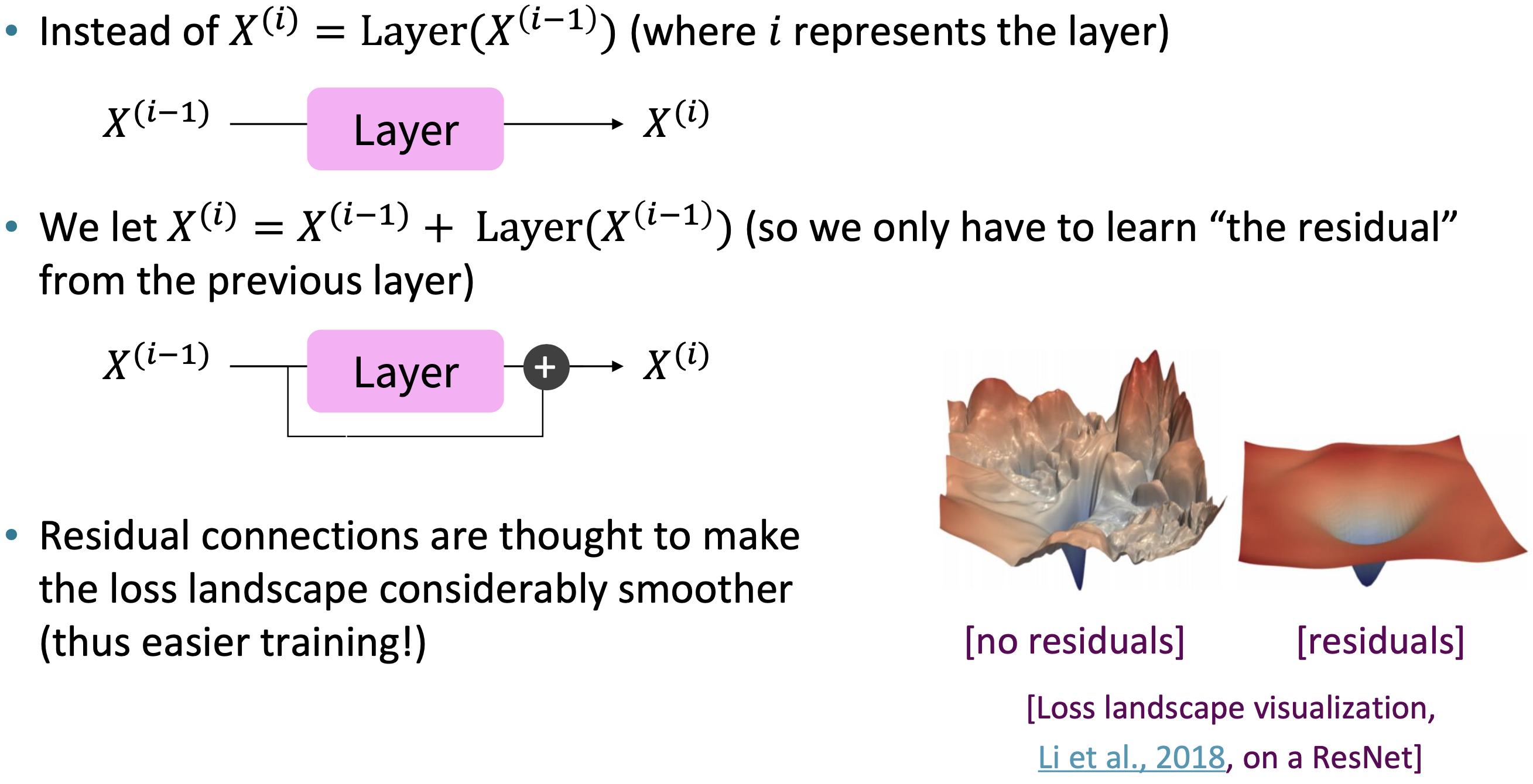
   Reference. Stanford CS224n, 2021, Li et al., 2018

2. Layer normalization, [Ba et al., 2016]
   • Layer normalization is a trick to help models train faster.
   • Idea: cut down on uninformative variation in hidden vector values by normalizing to unit mean and standard deviation within each layer.
   • LayerNorm’s success may be due to its normalizing gradients [Xu et al., 2019]
   \[\begin{aligned} &\text{Let } 𝑥 \in \mathbb{R}^𝑑\text{ be an individual (word) vector in the model.}\\ &\text{Let } \mu = \sum_{j=1}^d x_j;\text{ this is the mean}; \mu \in \mathbb{R}.\\ &\text{Let } \sigma = \sqrt{\frac{1}{d}\sum_{j=1}^d(x_j-\mu)^2};\text{ this is the standard deviation}; \sigma \in \mathbb{R}.\\\\ &\text{Let } \gamma \in \mathbb{R}^d and \beta \in \mathbb{R}^d\text{ be learned "gain" and "bias" parameters (Can omit)} \end{aligned}\]

   Then layer normalization computes:

   \[\text{output} = \dfrac{x - \mu}{\sqrt{\sigma}+\epsilon} * \gamma + \beta\] \[\begin{aligned} &\sigma,\text{ Normalize by scalar mean and variance} \\ &\gamma, \beta,\text{ Modulate by learned elementwise gain and bias} \\ \end{aligned}\]

3. Scaling the dot product

   “Scaled Dot Product” attention is a final variation to aid in Transformer training. When dimensionality 𝑑 becomes large, dot products between vectors tend to become large. Because of this, inputs to the softmax function can be large, making the gradients small.

   Instead of the self-attention function we’ve seen:

   \[output_{\ell} = softmax(XQ_{\ell}K_{\ell}^T X^T)*XV_{\ell}\]

   We divide the attention scores by $\sqrt{d/h}$, to stop the scores from becoming large just as a function of $d/h$ (The dimensionality divided by the number of heads.)

   \[output_{\ell} = softmax(\dfrac{XQ_{\ell}K_{\ell}^T X^T}{\sqrt{d/h}})*XV_{\ell}\]
4. These tricks don’t improve what the model is able to do; they help improve the training process. Both of these types of modeling improvements are very important!

4.2 Transformer Encoder-Decoder

Looking back at the whole model, zooming in on an Encoder block:

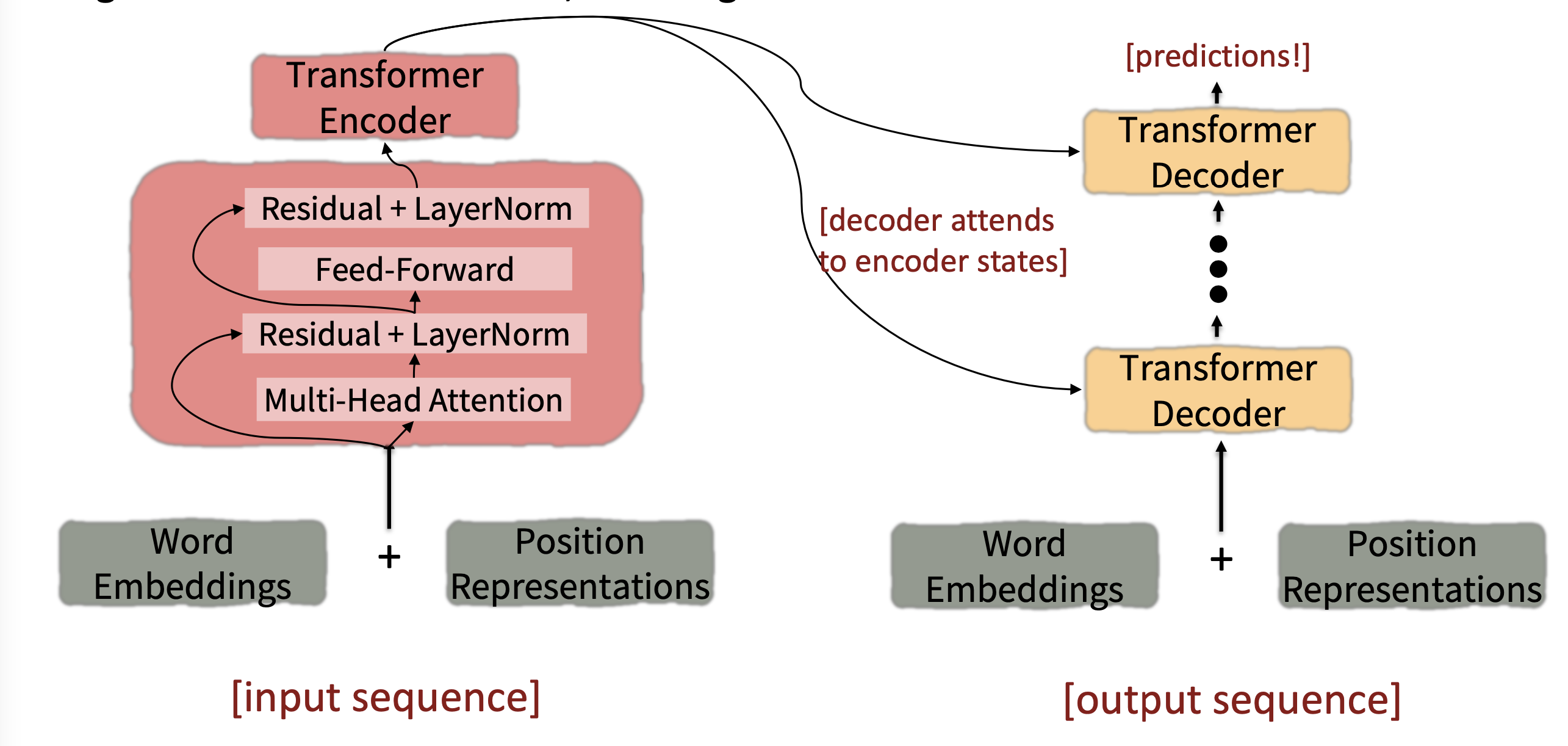
Reference. Stanford CS224n

Looking back at the whole model, zooming in on a Decoder block:

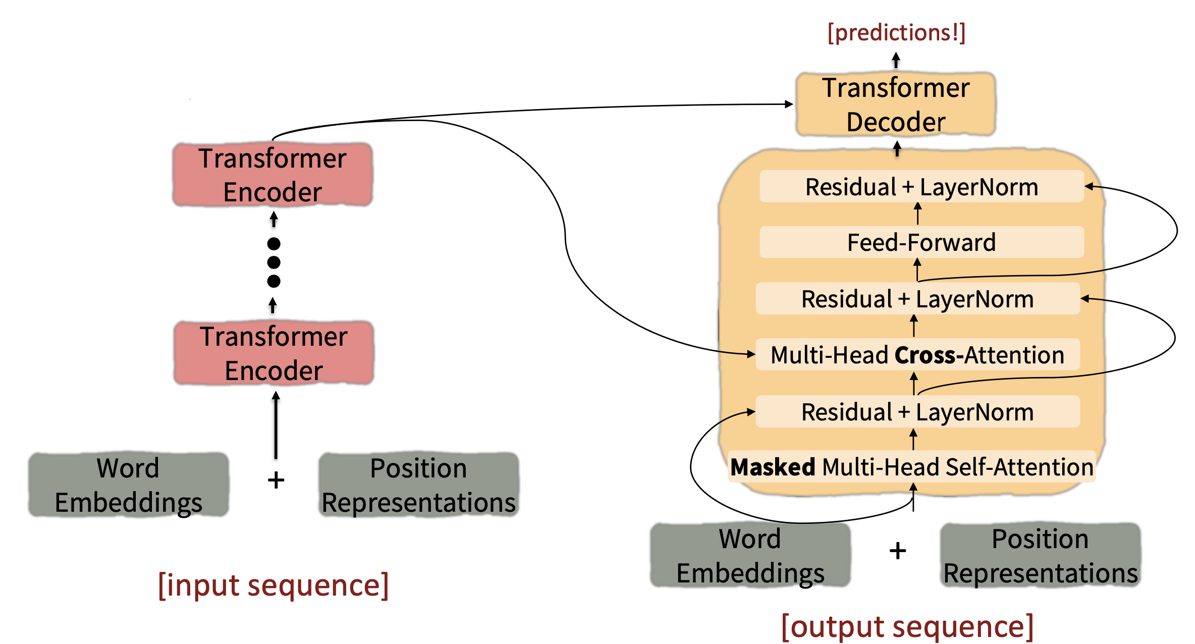
Reference. Stanford CS224n

The only new part is attention from decoder to encoder(Multi-Head Cross-Attention and Residual+LayerNorm)

4.3 Cross-attention

• We saw that self-attention is when keys, queries, and values come from the same source.
• Let $h_1, \dots , h_𝑇$ be output vectors from the Transformer encoder; $𝑥_𝑖 \in \mathbb{R}^𝑑$
• Let $𝑧_1 , \dots , 𝑧_T$ be input vectors from the Transformer decoder, $𝑧 \in \mathbb{R}^𝑑$

• Then keys and values are drawn from the encoder (like a memory):

  \[k_i=Kh_i,\ v_i=Vh_i\]
• And the queries are drawn from the decoder, $q_i=Qz_i$

• Let’s look at how cross-attention is computed, in matrices.

  \[\begin{aligned} &\text{Let }H = [h_1; \dots ; h_𝑇] \in \mathbb{R}^{𝑇\times d}\text{ be the concatenation of encoder vectors.}\\ &\text{Let }Z = [z_1; \dots ; z_𝑇] \in \mathbb{R}^{𝑇\times d}\text{ be the concatenation of decoder vectors.} \end{aligned}\] \[output = softmax(𝑍𝑄(𝐻𝐾)^⊤)×𝐻𝑉\]
• First, take the query-key dot products in one matrix multiplication: $𝑍𝑄(𝐻𝐾)^⊤$. Next, softmax, and compute the weighted average with another matrix multiplication.

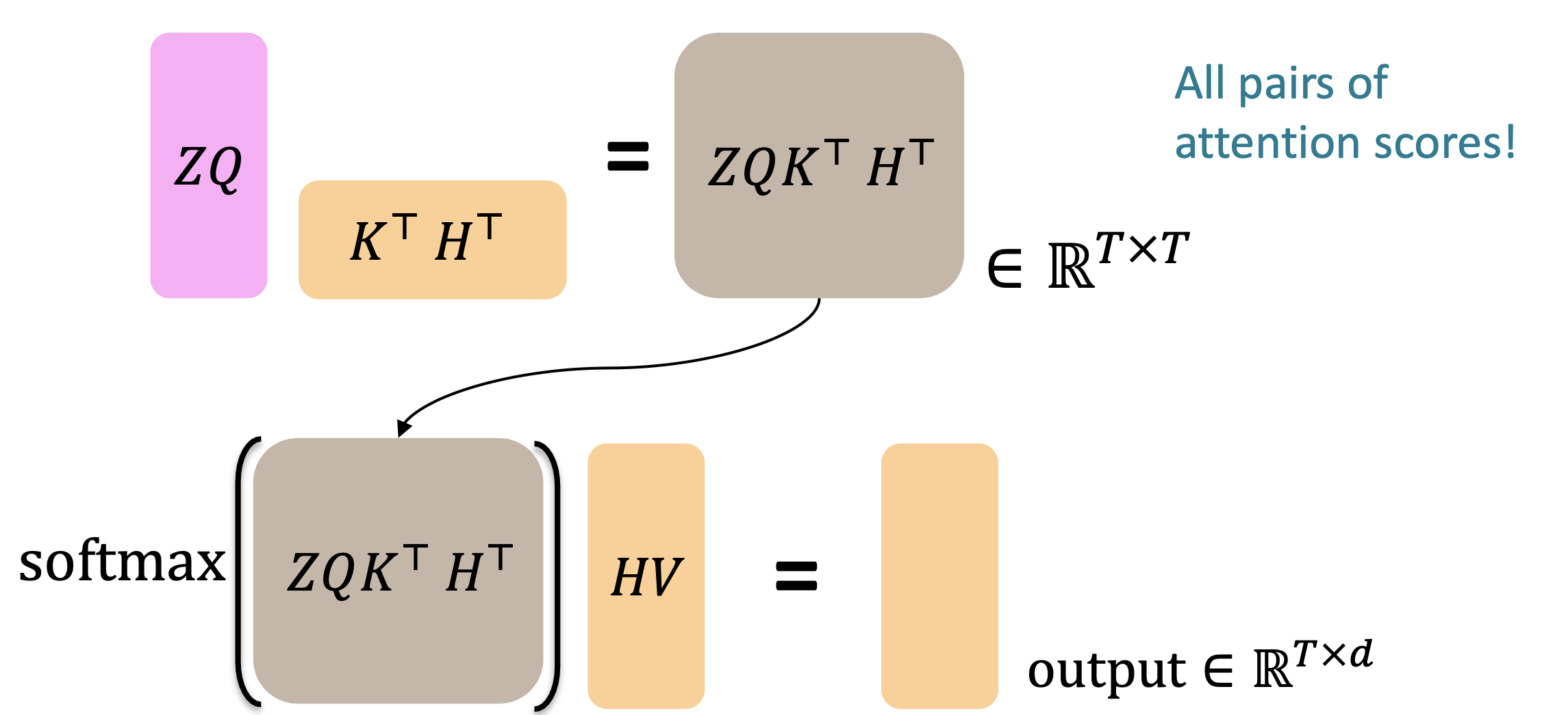
Reference. Stanford CS224n

4.4 Recent work

• Quadratic compute in self-attention (today):
  • Computing all pairs of interactions means our computation grows quadratically with the sequence length!
  • For recurrent models, it only grew linearly!
• Position representations

• Recent work on improving on quadratic self-attention cost

  Considerable recent work has gone into the question, Can we build models like Transformers without paying the $𝑂(𝑇^2)$ all-pairs self-attention cost?

  For example, BigBird [Zaheer et al., 2021]

  Key idea: replace all-pairs interactions with a family of other interactions, like local windows, looking at everything, and random interactions.

  

  Reference. Stanford CS224n

5. Pre-training

5.1 Brief overview

$\checkmark$ Word structure and subword models

Let’s take a look at the assumptions we’ve made about a language’s vocabulary. We assume a fixed vocab of tens of thousands of words, built from the training set. All novel words seen at test time are mapped to a single UNK.

Reference. Stanford CS224n

Finite vocabulary assumptions make even less sense in many languages. Many languages exhibit complex morphology, or word structure.

• The effect is more word types, each occurring fewer times.

Example: Swahili verbs can have hundreds of conjugations, each encoding a wide variety of information. (Tense, mood, definiteness, negation, information about the object, ++)

$\checkmark$ The byte-pair encoding algorithm

Subword modeling in NLP encompasses a wide range of methods for reasoning about structure below the word level. (Parts of words, characters, bytes.)

• The dominant modern paradigm is to learn a vocabulary of parts of words (subword tokens).

• At training and testing time, each word is split into a sequence of known subwords.

  Byte-pair encoding is a simple, effective strategy for defining a subword vocabulary.

  1. Start with a vocabulary containing only characters and an “end-of-word” symbol.
  2. Using a corpus of text, find the most common adjacent characters “a,b”; add “ab” as a subword.
  3. Replace instances of the character pair with the new subword; repeat until desired vocab size.

  Originally used in NLP for machine translation; now a similar method (WordPiece) is used in pretrained models.

Common words end up being a part of the subword vocabulary, while rarer words are split into (sometimes intuitive, sometimes not) components.

In the worst case, words are split into as many subwords as they have characters.

Reference. Stanford CS224n

$\checkmark$ Motivating model pretraining from word embeddings

Recall the adage we mentioned at the beginning of the course:

“You shall know a word by the company it keeps” (J. R. Firth 1957: 11)

This quote is a summary of distributional semantics, and motivated word2vec. But:

“... the complete meaning of a word is always contextual,

and no study of meaning apart from a complete context 

can be taken seriously.” (J. R. Firth 1935)

Consider I record the record*: the two instances of record mean different things.

$\checkmark$ Where we were: pretrained word embeddings, Circa 2017

• Start with pretrained word embeddings (no context!)
• Learn how to incorporate context in an LSTM or Transformer while training on the task.

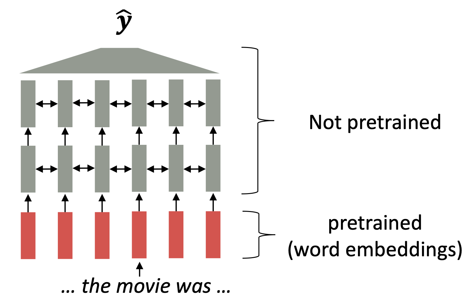
Reference. Stanford CS224n, Recall, movie gets the same word embedding, no matter what sentence it shows up in

$\checkmark$ Some issues to think about:

1. The training data we have for our downstream task (like question answering) must be sufficient to teach all contextual aspects of language.
2. Most of the parameters in our network are randomly initialized!

In modern NLP:

• All (or almost all) parameters in NLP networks are initialized via pretraining.
• Pretraining methods hide parts of the input from the model, and train the model to reconstruct those parts.

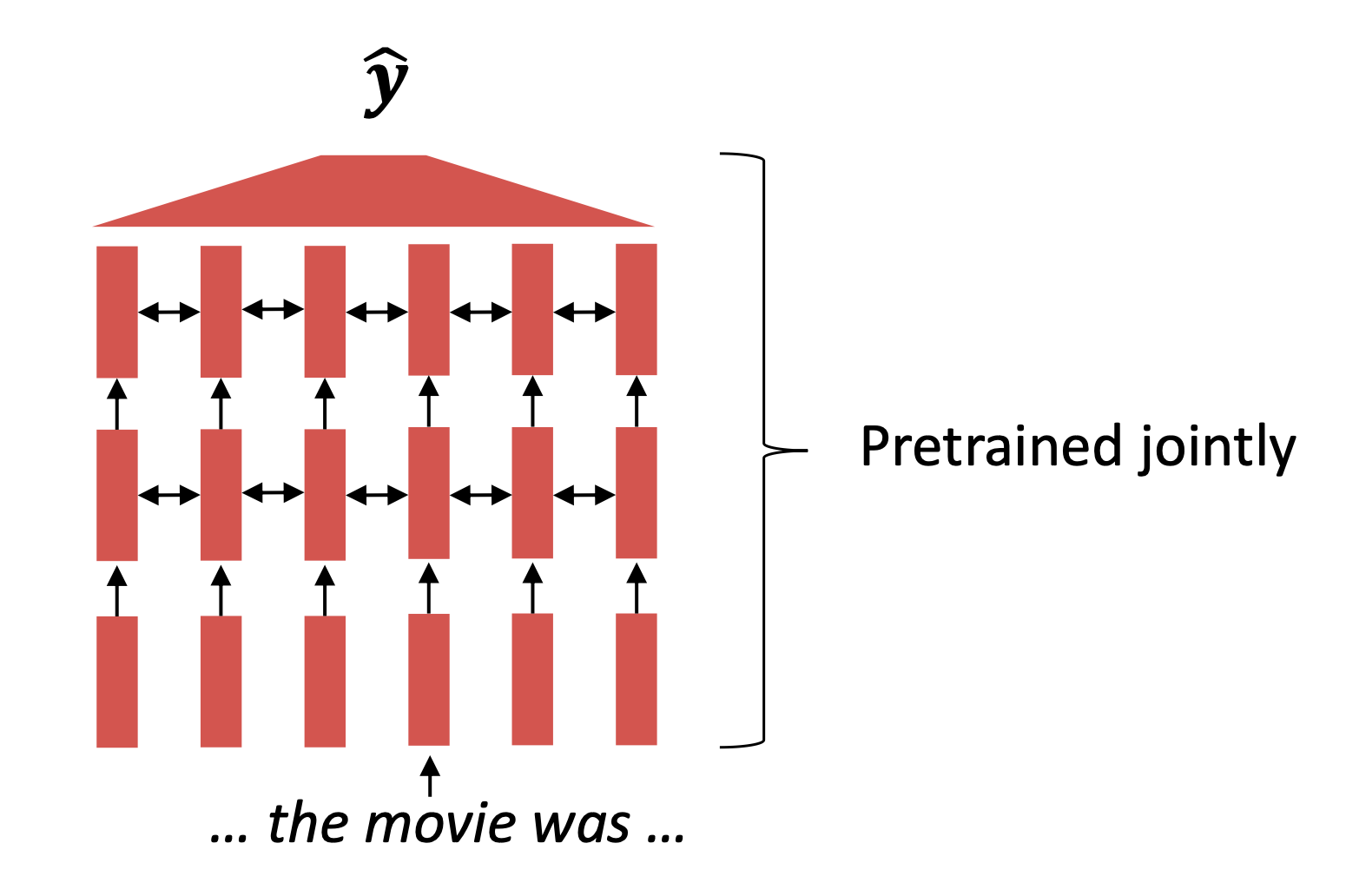
Reference. Stanford CS224n, This model has learned how to represent entire sentences through pretraining

• This has been exceptionally effective at building strong:
  • representations of language
  • parameter initializations for strong NLP models.
  • Probability distributions over language that we can sample from

Recall the language modeling task:

• Model $p_{\theta}(w_t\lvert w_{1:t-1})$, the probability distribution over words given their past contexts.

  

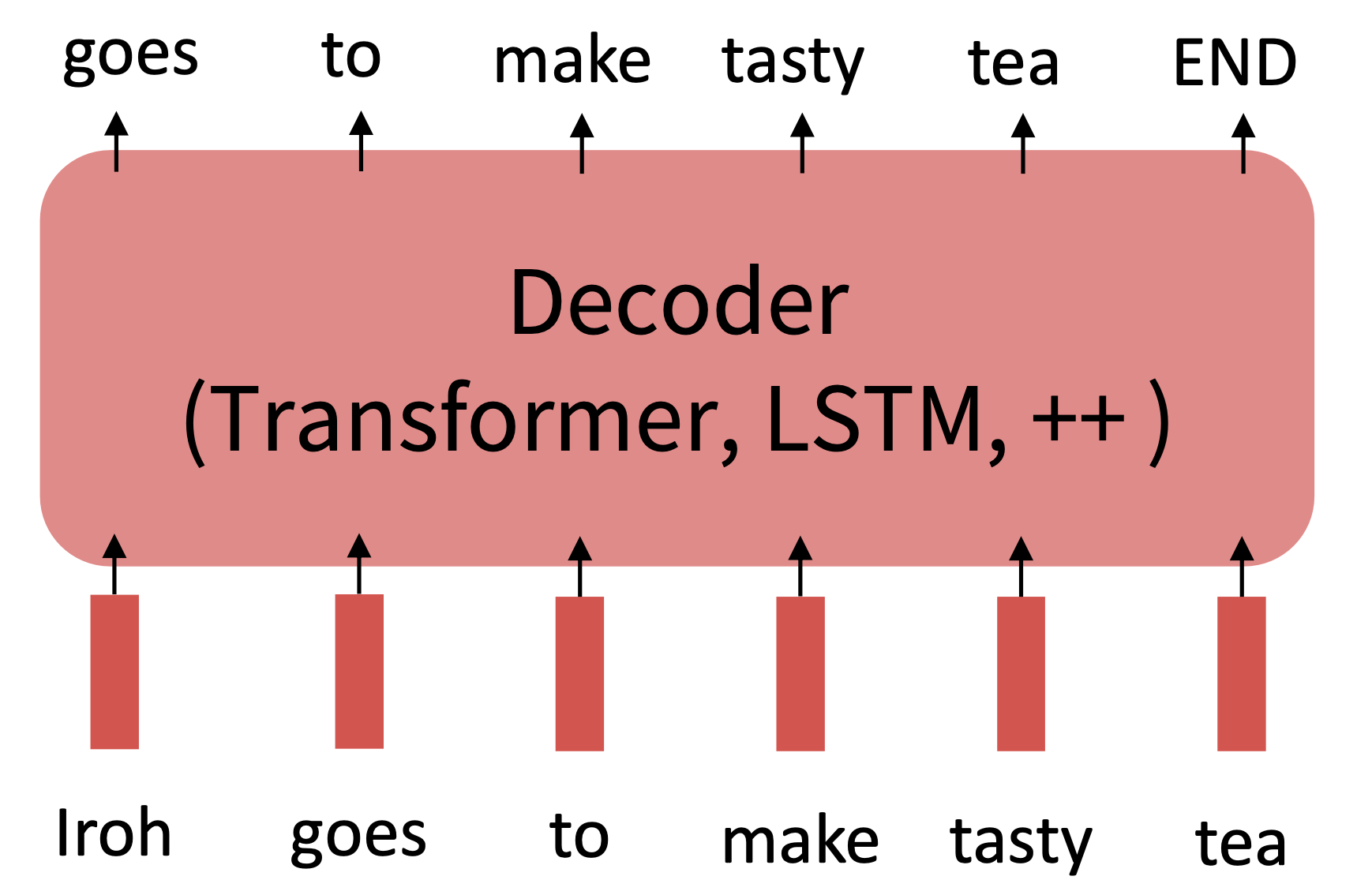
  Reference. Stanford CS224n, Step 1: Pretrain (on language modeling)

$\checkmark$ Pretraining through language modeling [Dai and Le, 2015]

• Train a neural network to perform language modeling on a large amount of text.
• Save the network parameters.

Pretraining can improve NLP applications by serving as parameter initialization.

• Step 1: Pretrain (on language modeling): Lots of text; learn general things!

• Step 2: Finetune (on your task) Not many labels; adapt to the task!

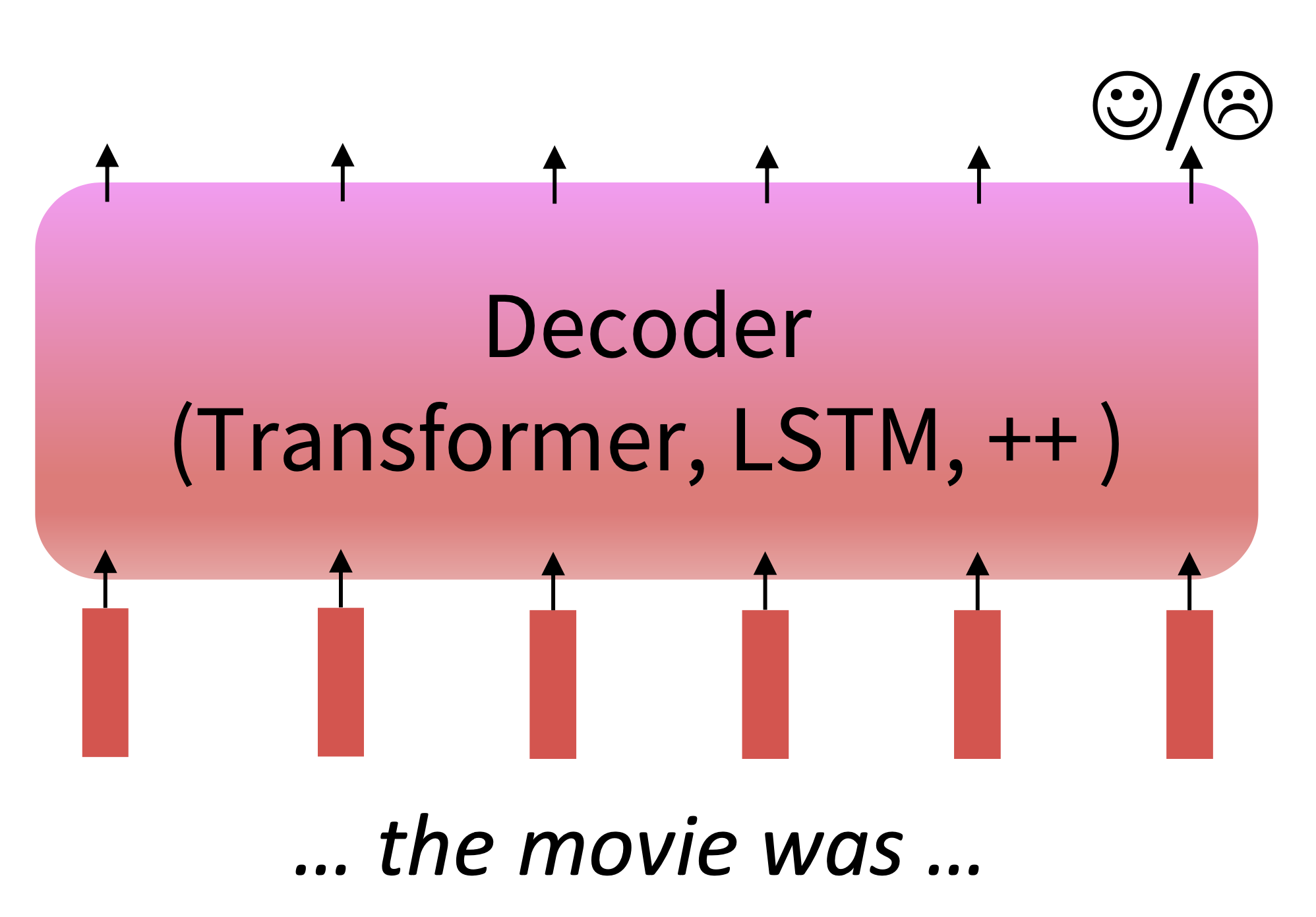
Reference. Stanford CS224n, Step 1: Pretrain (on language modeling)

Why should pretraining and finetuning help, from a “training neural nets” perspective? Consider, provides parameters $\hat \theta$ by approximating $\underset{\theta}{min}\ L_{pretrain}(\theta)$, pretrain loss. Then, finetuning approximates $\underset{\theta}{min}\ L_{finetune}(\theta)$, starting at $\hat \theta$, finetuning loss. The pretraining may matter because stochastic gradient descent sticks (relatively) close to $\hat \theta$ during finetuning.

• So, maybe the finetuning local minima near $\hat \theta$ tend to generalize well!
• And/or, maybe the gradients of finetuning loss near $\hat \theta$ propagate nicely!

5.2 Model Pretraining ways

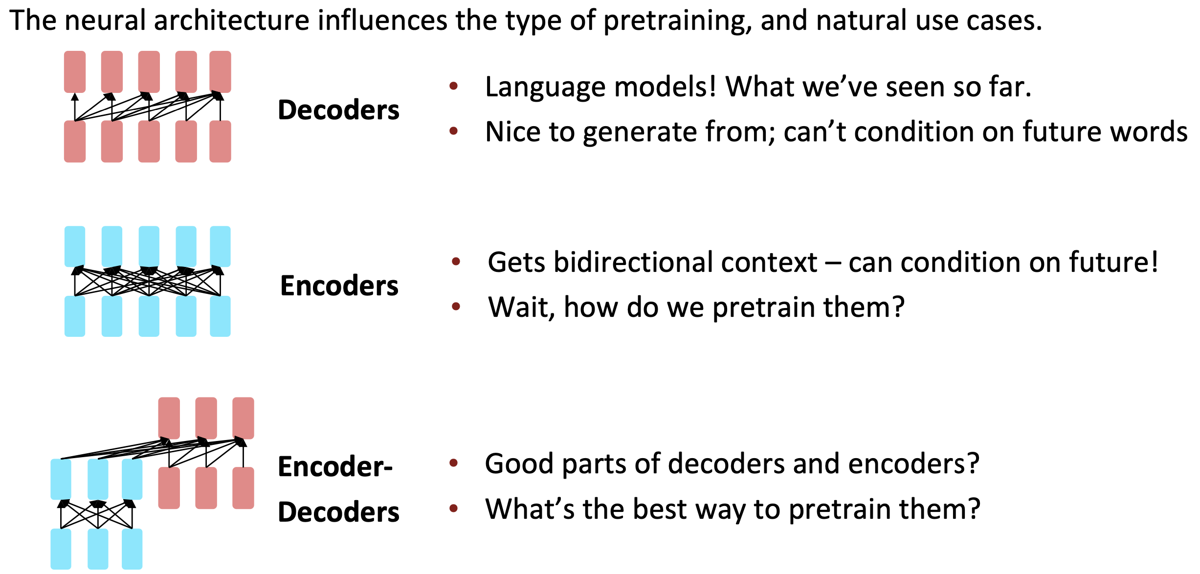
Reference. Stanford CS224n, 2021

$\checkmark$ #1 Decoders

1. Pretraining

   When using language model pretrained decoders, we can ignore that they were trained to model $p(w_t\lvert w_{1:t-1})$. We can fine-tune them by training a classifier on the lsat word’s hidden state.

   

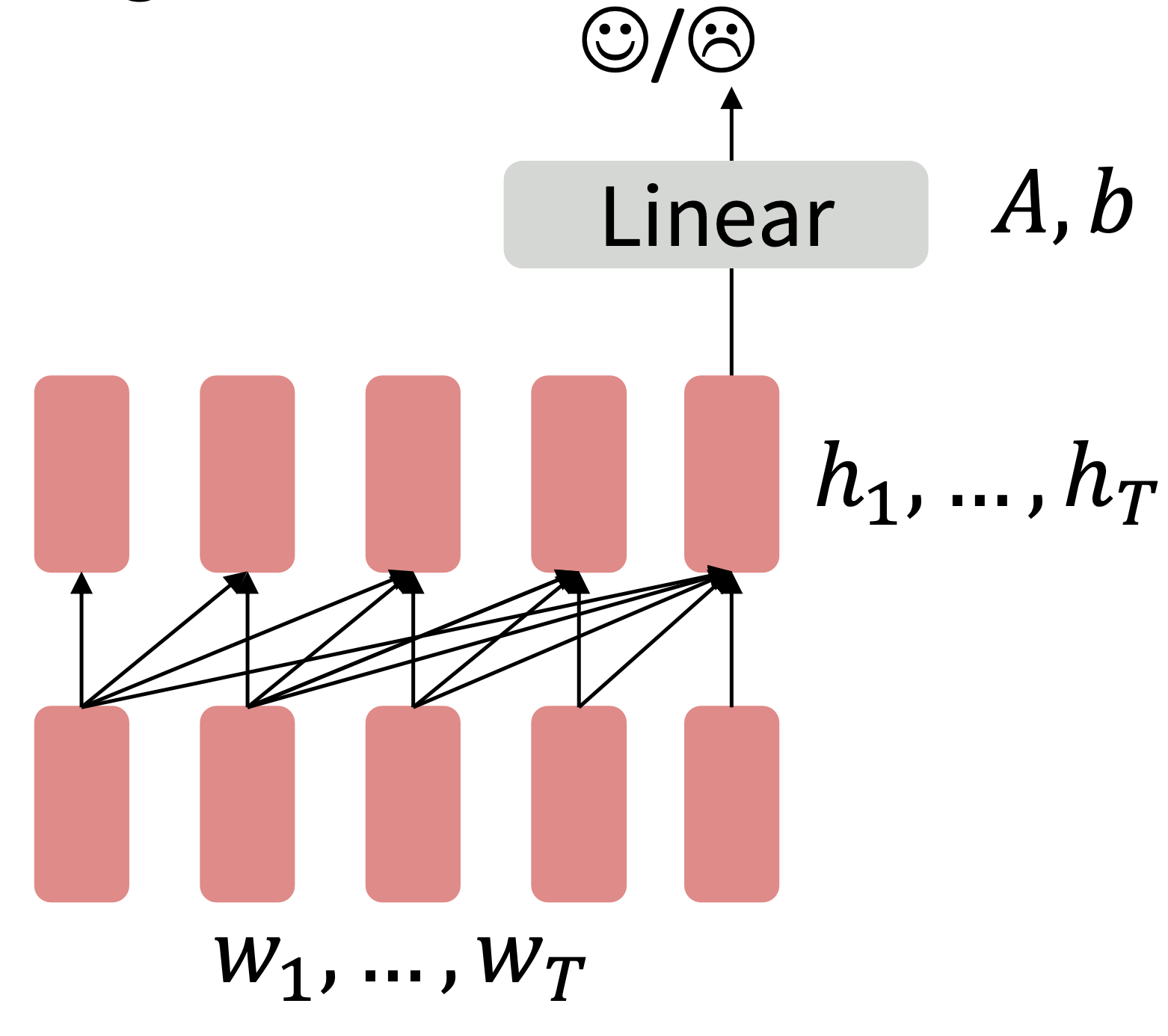
   Reference. Stanford CS224n, 2021, Note how the linear layer hasn’t been pretrained and must be learned from scratch.

   \[h_1, \dots, h_T = Decoder(w_1,\dots, w_T) \\ y\sim Aw_T +b\]

   Where A and b are randomly initialized and specified by the downstream task. Gradients backpropagate through the whole network.

2. Finetuning

   

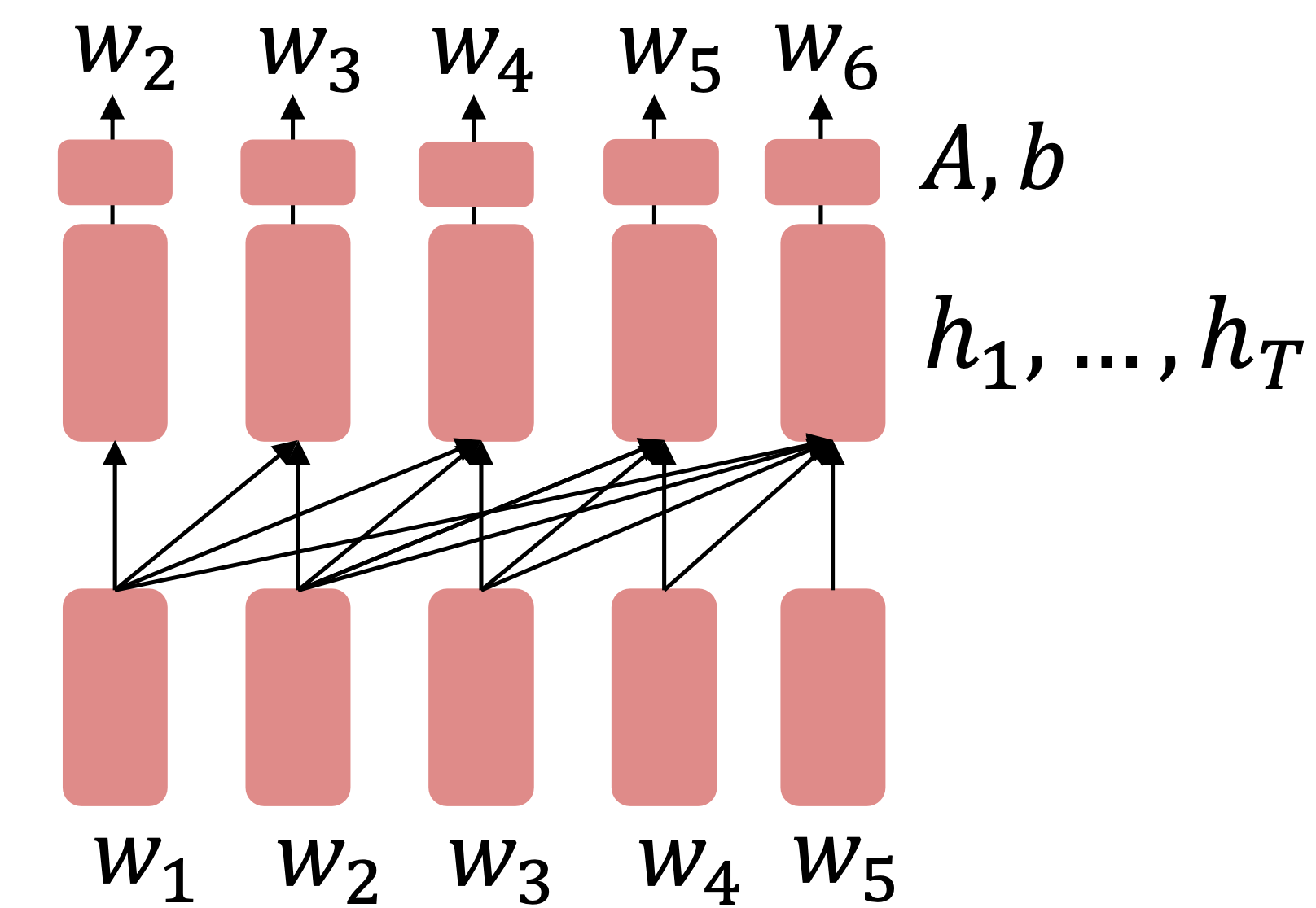
   Reference. Stanford CS224n, 2021, Note how the linear layer has been pretrained.

   It’s natural to pretrain decoders as language models and then use them as generators, finetuning their $p_{\theta}(w_t\lvert w_{1:t-1})$.

   This is helpful in tasks where the output is a sequence with a vocabulary like that at pretraining time.

   • Dialogue (context=dialogue history)
   • Summarization (context=document)
   \[h_1, \dots, h_T = Decoder(w_1,\dots, w_T) \\ w_t \sim Aw_{t-1} +b\]

   Where A, b were pretrained in the language model

$\checkmark$ Generative Pretrained Transformer (GPT) [Radford et al., 2018]

2018’s GPT was a big success in pretraining a decoder!

• Transformer decoder with 12 layers.
• 768-dimensional hidden states, 3072-dimensional feed-forward hidden layers.
• Byte-pair encoding with 40,000 merges

• Trained on BooksCorpus: over 7000 unique books.

  • Contains long spans of contiguous text, for learning long-distance dependencies.
• The acronym “GPT” never showed up in the original paper; it could stand for “Generative PreTraining” or “Generative PreTrained Transformer”

• How do we format inputs to our decoder for finetuning tasks?

  • Radford et al., 2018 evaluate on natural language inference.

  • Natural Language Inference: Label pairs of sentences as entailing/contradictory/neutral

  • Entailment

          Premise: The man is in the doorway 
          Hypothesis: The person is near the door
    

    Here’s roughly how the input was formatted, as a sequence of tokens for the decoder.

        [START] The man is in the doorway [DELIM] The person is near the door [EXTRACT]
  

  The linear classifier is applied to the representation of the [EXTRACT] token.

• Increasingly convincing generations (GPT2) [Radford et al., 2018]

  We mentioned how pretrained decoders can be used in their capacities as language models.

  GPT-2, a larger version of GPT trained on more data, was shown to produce relatively convincing samples of natural language.

$\checkmark$ #2 Encoders, Encoders get bidirectional context!

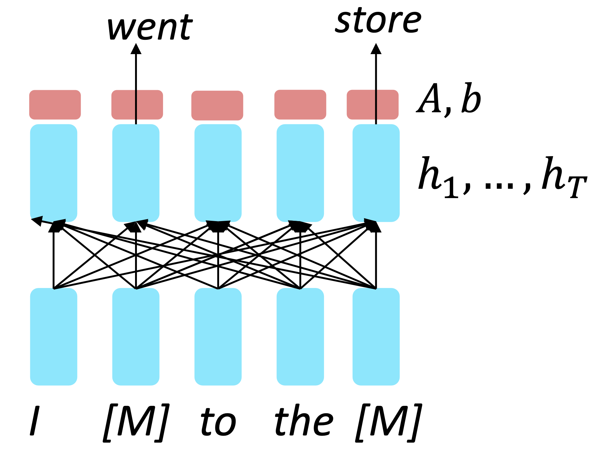
Reference. Devlin et al., 2018

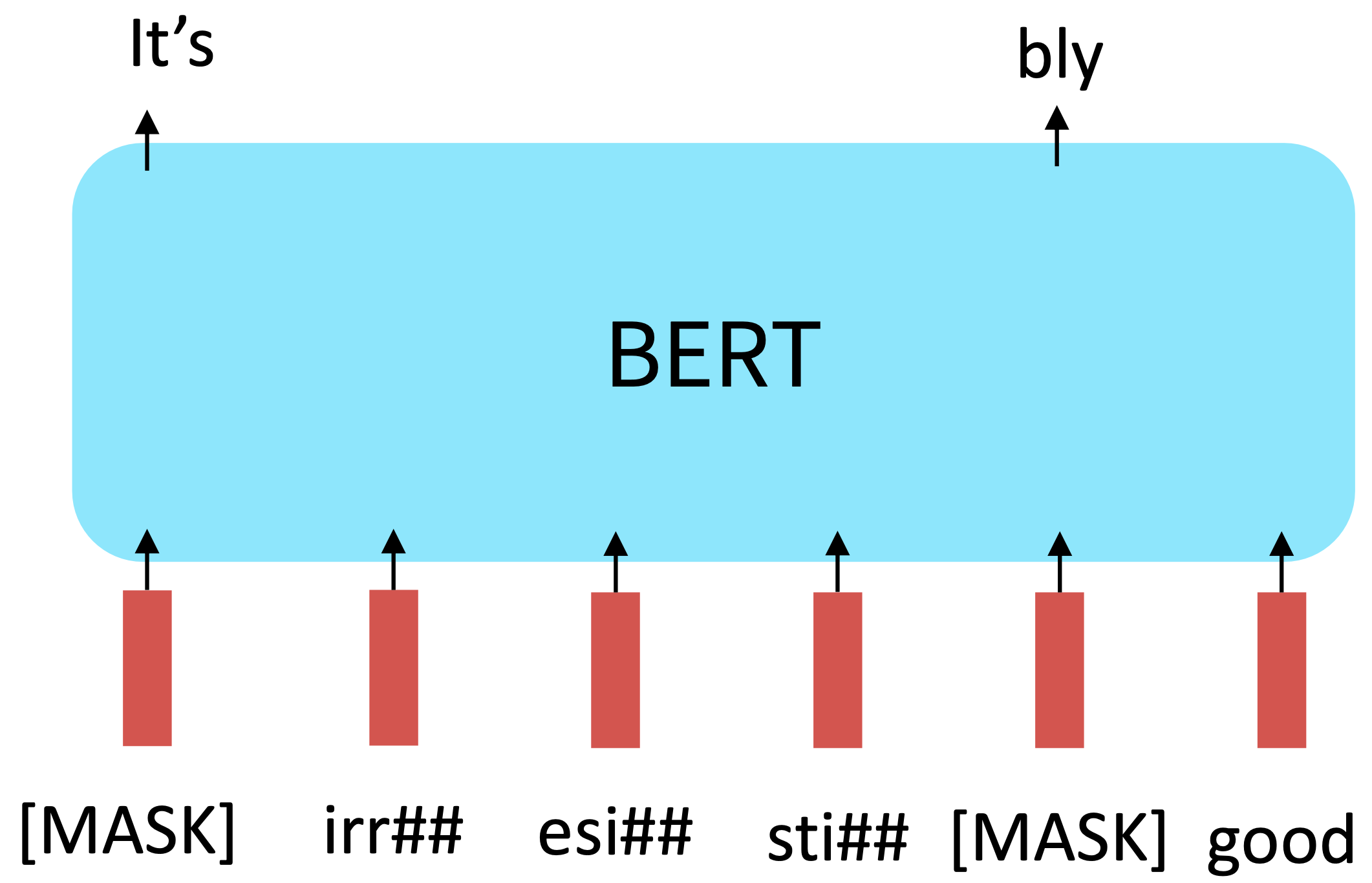
Idea: replace some fraction of words in the input with a special [MASK] token; predict these words.

Only add loss terms from words that are “masked out.” If $\tilde x$ is the masked version of x, we’re learning $p_{\theta}(x\lvert \tilde x)$. Called Masked LM.

$\checkmark$ BERT: Bidirectional Encoder Represetations from Transformers

Devlin et al., 2018 proposed the “Masked LM” objective and released the weights of a pretrained Transformer, a model they labeled BERT.

Some more details about Masked LM for BERT:

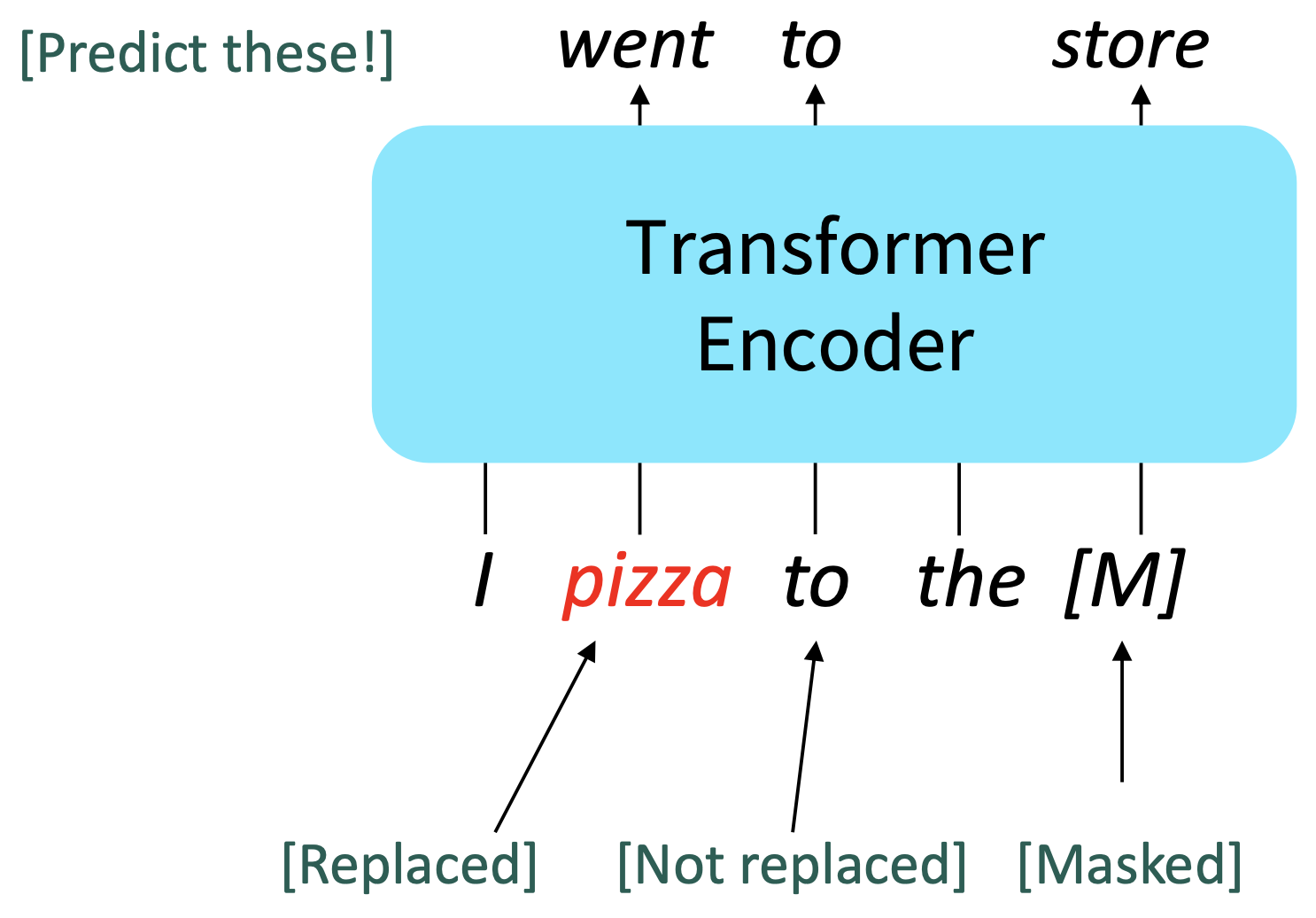
Reference. Devlin et al., 2018

• Predict a random 15% of (sub)word tokens.
  • Replace input word with [MASK] 80% of the time
  • Replace input word with a random token 10% of the time
  • Leave input word unchanged 10% of the time (but still predict it!)
• Why? Doesn’t let the model get complacent and not build strong representations of non-masked words. (No masks are seen at fine-tuning time!)

• The Pretraining input to BERT was two separate contiguous chunks of text: “Segment Embedding”, Devlin et al., 2018, Liu et al., 2019]

  

  Reference. Devlin et al., 2018, Liu et al., 2019

• BERT was trained to predict whether one chunk follows the other or is randomly sampled. Later work has argued this “next sentence prediction” is not necessary.

• Detail

  • Two models were released:

    BERT-base: 12 layers, 768-dim hidden states, 12 attention heads, 110 million params

    BERT-large: 24 layers, 1024-dim hidden states, 16 attention heads, 340 million params.

  • Trained on:

    BooksCorpus (800 million words)

    English Wikipedia (2,500 million words)

  • Pretraining is expensive and impractical on a single GPU.

    BERT was pretrained with 64 TPU chips for a total of 4 days. 

    TPUs are special tensor operation acceleration hardware)

  • Finetuning is practical and common on a single GPU

    “Pretrain once, finetune many times.”

  • Evaluation

    • QQP: Quora Question Pairs (detect paraphrase • questions)
    • QNLI: natural language inference over question answering data
    • SST-2: sentiment analysis
    • CoLA: corpus of linguistic acceptability (detect whether sentences are grammatical.)
    • STS-B: semantic textual similarity
    • MRPC: microsoft paraphrase corpus
    • RTE: a small natural language inference corpus

• Limitness

  If your task involves generating sequences, consider using a pretrained decoder; BERT and other pretrained encoders don’t naturally lead to nice autoregressive (1-word-at-a-time) generation methods.

  

  Reference. Stanford CS224n

• Expansions of BERT

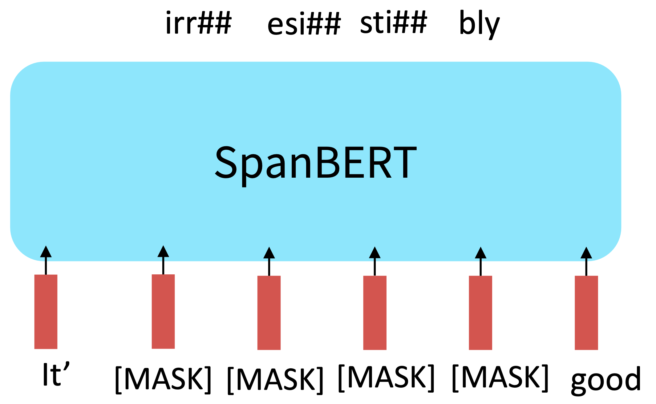
  RoBERTa, SpanBERT, +++

  1. RoBERTa: mainly just train BERT for longer and remove next sentence prediction!, Liu et al., 2019

     

     Reference. Liu et al., 2019

  2. SpanBERT: masking contiguous spans of words makes a harder, more useful pretraining task, Joshi et al., 2020

     

     Reference. Joshi et al., 2020

$\checkmark$#3 Encoder-Decoders

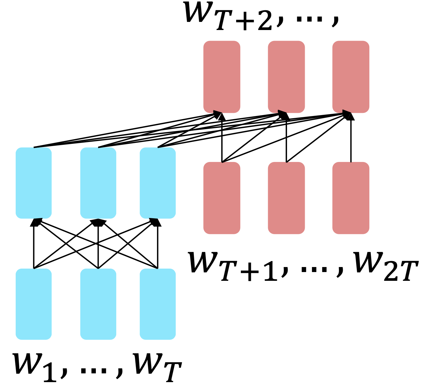
For encoder-decoders, we could do something like language modeling, but where a prefix of every input is provided to the encoder and is not predicted.

Reference. Raffel et al., 2018

The encoder portion benefits from bidirectional context; the decoder portion is used to train the whole model through language modeling.

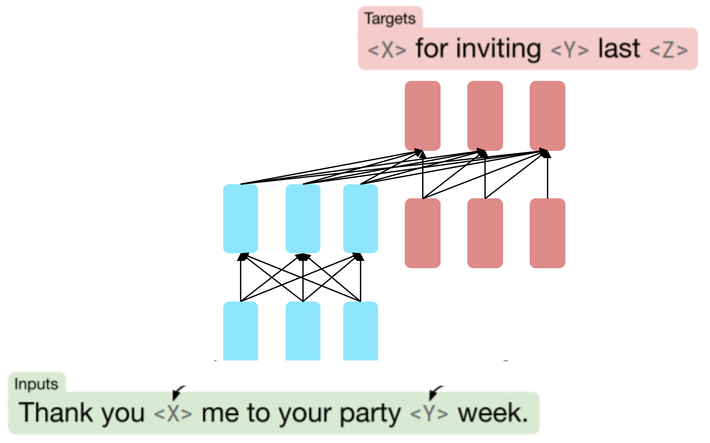
What Raffel et al., 2018 found to work best was span corruption. Their model: T5 , which replaces different-length spans from the input with unique placeholders; decode out the spans that were removed

Reference. Raffel et al., 2018

This is implemented in text preprocessing: it’s still an objective that looks like language modeling at the decoder side.

A fascinating property of T5: it can be finetuned to answer a wide range of questions, retrieving knowledge from its parameters.

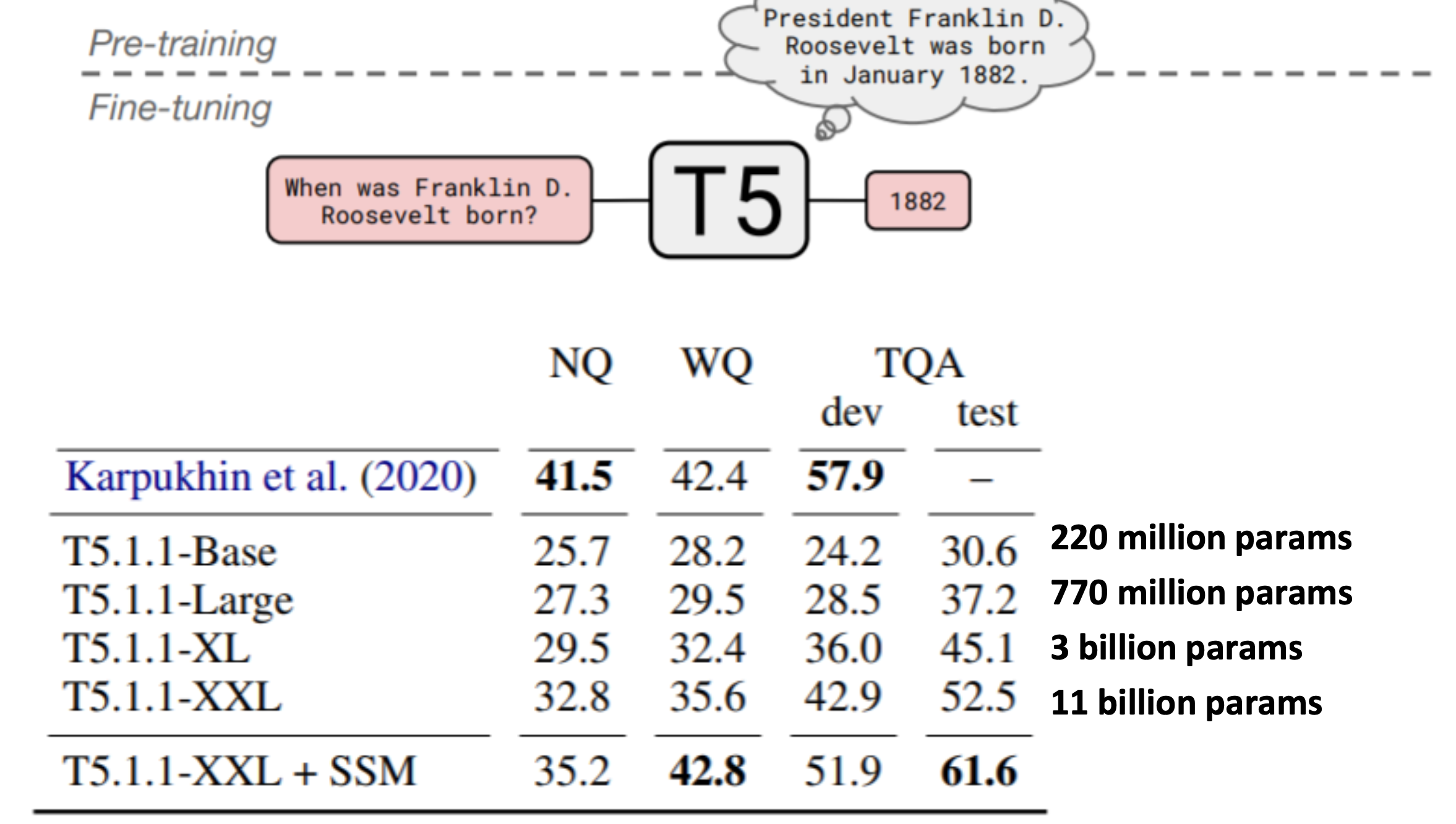
Reference. Raffel et al., 2018, NQ: Natural Questions, WQ: WebQuestions, TQA: Trivia QA, All "open-domain" versions

6. GPT-3, In-context learning, and very large models

Very large language models seem to perform some kind of learning without gradient steps simply from examples you provide within their contexts. GPT-3 is the canonical example of this. The largest T5 model had 11 billion parameters. GPT-3 has 175 billion parameters.

The in-context examples seem to specify the task to be performed, and the conditional distribution mocks performing the task to a certain extent.

Input (prefix within a single Transformer decoder context):

" thanks → merci

    hello → bonjour 

    mint → menthe

    otter →               " 

Output (conditional generations):

loutre..."

Very large language models seem to perform some kind of learning without gradient steps simply from examples you provide within their contexts.

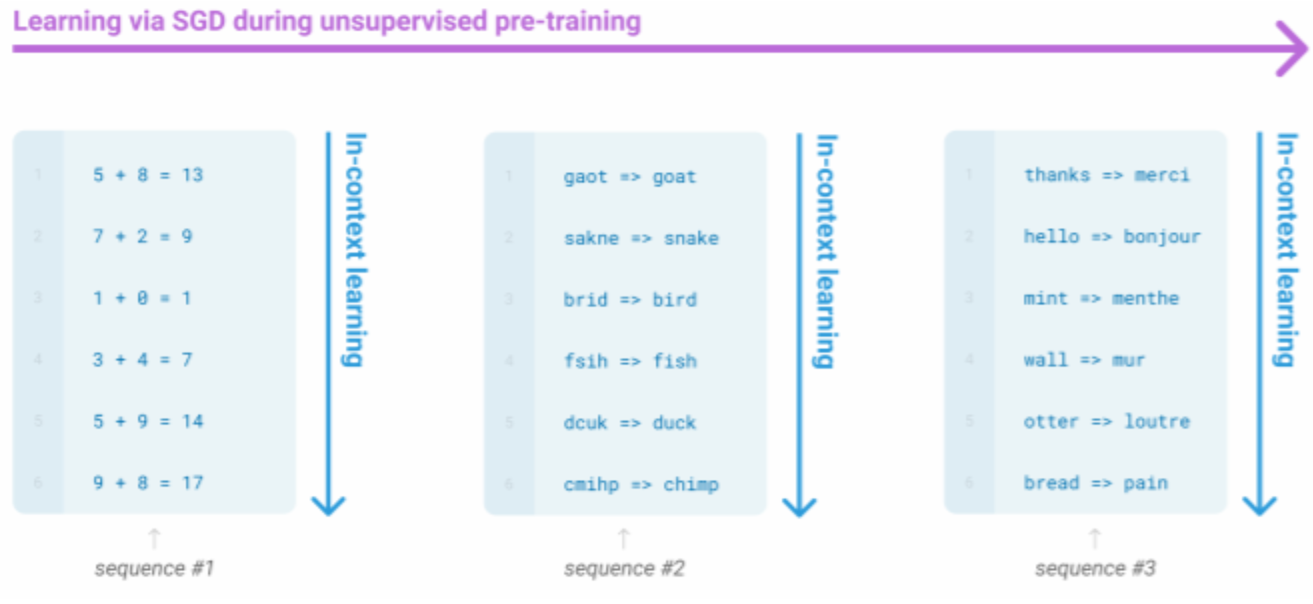
Reference. Stanford CS224n