CS224N W4. Machine Translation Sequence to Sequence And Attention

All contents is arranged from CS224N contents. Please see the details to the CS224N!

1. Statistical Machine Translation, SMT (1990s-2010s)

“Learn a probabilistic model from data”

it want to find best English sentence y, given French sentence x.

\[argmax_y P(y\lvert x)\]

Use Bayes Rule to break this down into two components to be learned separately:

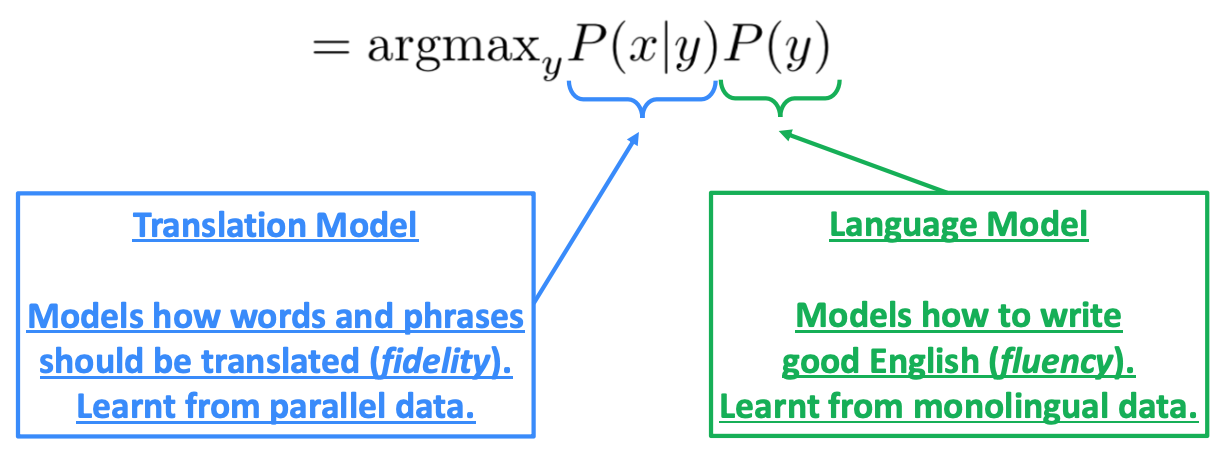
Reference. Stanford CS224n, 2021

It needs large amount of parallel data(e.g. pairs of human-translated French/English sentences). Break it down further: Introduce latent a variable into the model: $P(x, a\lvert y)$, where a is the alignment, i.e. word-level correspondence between source sentence x and target sentence y. Alignment is the correspondence between particular words in the translated sentence pair. Typological differences between languages lead to complicated alignments! Note: Some words have no counterpart. Alignment can be many-to-one or one-to-many or many-to-many (phrase-level).

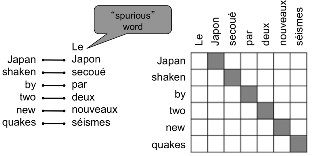
Reference. Stanford CS224n, 2021, Examples from: “The Mathematics of Statistical Machine Translation: Parameter Estimation", Brown et al, 1993.

1.1 Learning alignment for SMT

We learn as a combination of many factors, including:

Probability of particular words aligning (also depends on position in sent)
Probability of particular words having a particular fertility (number of corresponding words)
etc.

Alignments $a$ are latent variables: They aren’t explicitly specified in the data!

Require the use of special learning algorithms (like Expectation-Maximization) for learning the parameters of distributions with latent variables

1.2 Decoding for SMT

Reference. Stanford CS224n, 2021

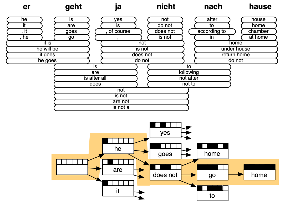
Reference. Stanford CS224n, 2021, ”Statistical Machine Translation", Chapter 6, Koehn, 2009.

$\checkmark$ The best systems were extremely complex

Hundreds of important details Systems had many separately-designed subcomponents
Lots of feature engineering such as need to design features to capture particular language phenomena
Require compiling and maintaining extra resources
Lots of human effort to maintain

$\checkmark$ Refernece

2. Neural Machine Translation

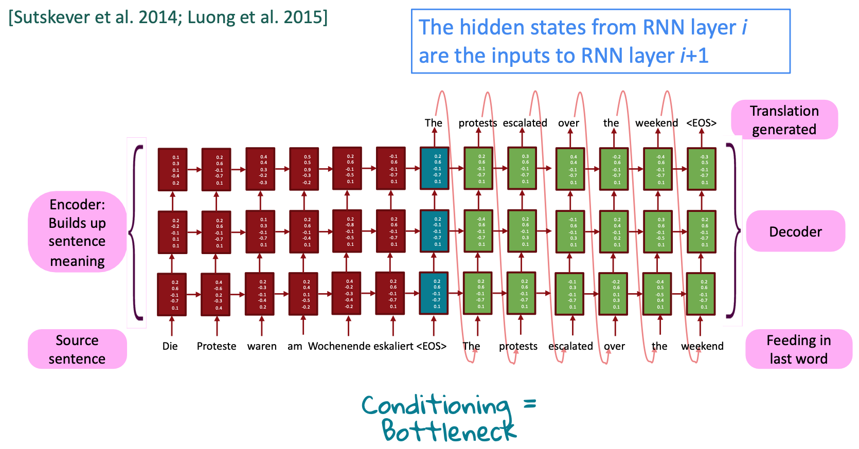
Neural Machine Translation (NMT) is a way to do Machine Translation with a single end-to-end neural network. The neural network architecture is called a sequence-to-sequence model (aka seq2seq) and it involves two RNNs

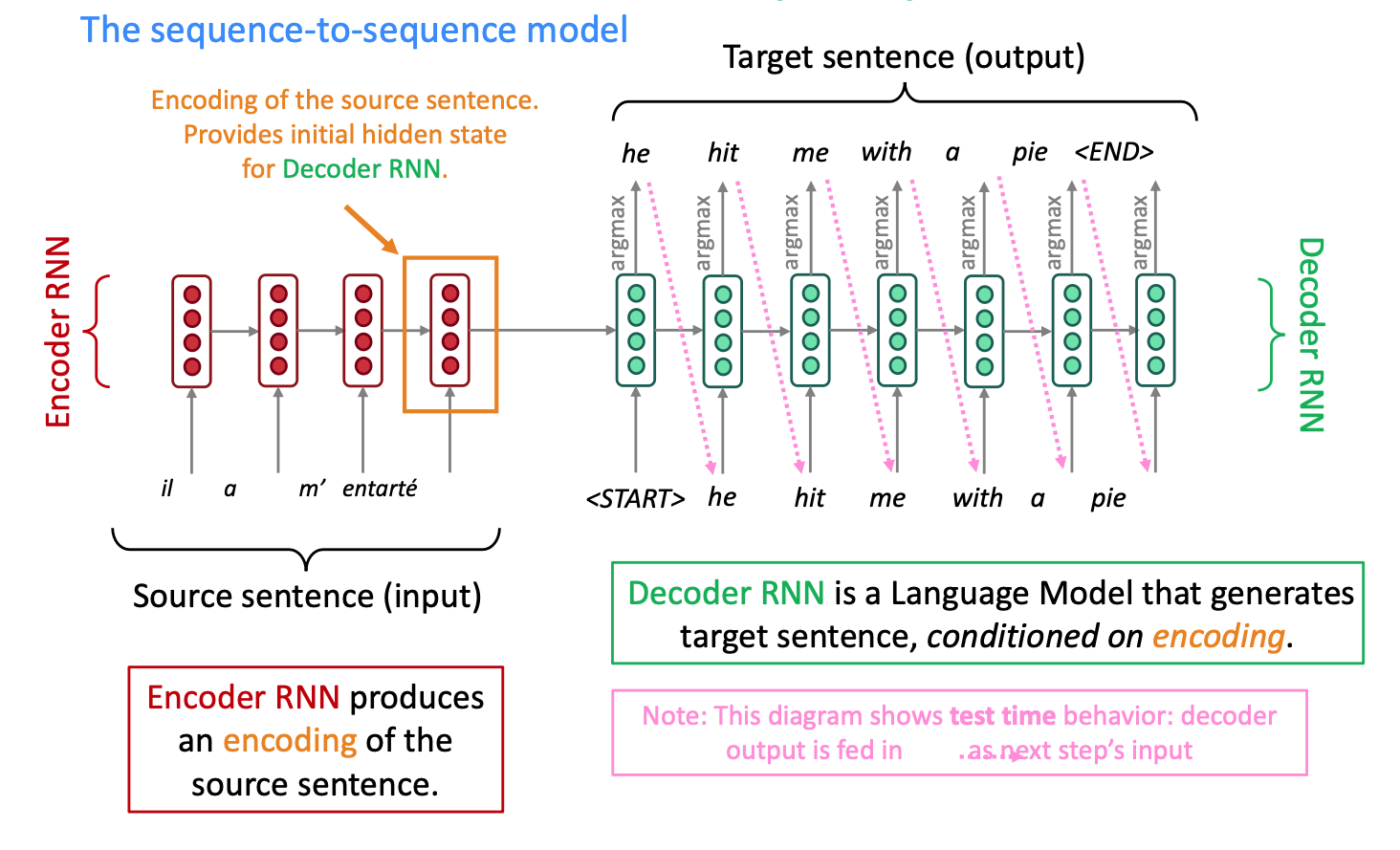
Reference. Stanford CS224n, 2021

Many NLP tasks can be phrased as sequence-to-sequence:

Summarization (long text → short text)
Dialogue (previous utterances → next utterance)
Parsing (input text → output parse as sequence)
Code generation (natural language → Python code)

The sequence-to-sequence model is an example of a Conditional Language Model.

NMT directly calculates $P(y\lvert x)=P(y_1\lvert x)P(y_2\lvert y_1,x)…P(y_t\lvert y_1,…,y_{t-1},x)$

2.1 Training a Neural Machine Translation system

Reference. Stanford CS224n, 2021

2.2 Sequence to Sequence basics

Sequence-to-sequence, or “Seq2Seq”, is a relatively new paradigm, with its first published usage in 2014 for English-French translation. At a high level, a sequence-to-sequence model is an end-to-end model made up of two recurrent neural networks:

an encoder, which takes the model’s input sequence as input and encodes it into a fixed-size “context vector”, and
a decoder, which uses the context vector from above as a “seed” from which to generate an output sequence.

For this reason, Seq2Seq models are often referred to as encoder-decoder models.

$\checkmark$ Encoder

The encoder network’s job is to read the input sequence to our Seq2Seq model and generate a fixed-dimensional context vector $C$ for the sequence. To do so, the encoder will use a recurrent neural network cell – usually an LSTM – to read the input tokens one at a time. The final hidden state of the cell will then become $C$. However, because it’s so difficult to compress an arbitrary-length sequence into a single fixed-size vector (especially for difficult tasks like translation), the encoder will usually consist of stacked LSTMs: a series of LSTM “layers” where each layer’s outputs are the input sequence to the next layer. The final layer’s LSTM hidden state will be used as $C$.

Seq2Seq encoders will often do something strange: they will process the input sequence in reverse. This is actually done on purpose. The idea is that, by doing this, the last thing that the encoder sees will (roughly) corresponds to the first thing that the model outputs; this makes it easier for the decoder to “get started” on the output, which **makes then gives the decoder an easier time generating a proper output sentence. In the context of translation, we’re allowing the network to translate the first few words of the input as soon as it sees them; once it has the first few words translated correctly, it’s much easier to go on to construct a correct sentence than it is to do so from scratch. See below figure for an example of what such an encoder network might look like.

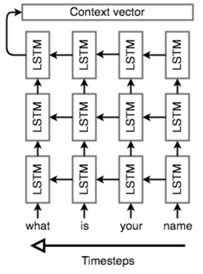
Reference. Stanford CS224n, 2021, Figure : Example of a Seq2Seq encoder network. This model may be used to translate the English sentence "whatis your name?" Note that the input tokens are read in reverse. Note that the network is unrolled; each column is a timestep and each row is a single layer, so that horizontal arrows correspond to hidden states and vertical arrows are LSTM inputs/outputs.

$\checkmark$ Decoder

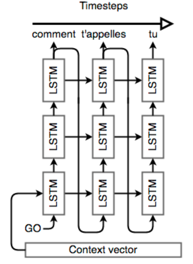
The decoder is also an LSTM network, but its usage is a little more complex than the encoder network. Essentially, we’d like to use it as a language model that’s “aware” of the words that it’s generated so far and of the input. To that end, we’ll keep the “stacked” LSTM architecture from the encoder, but we’ll initialize the hidden state of our first layer with the context vector from above; the decoder will literally use the context of the input to generate an output.

Once the decoder is set up with its context, we’ll pass in a special token to signify the start of output generation; in literature, **this is usually an token appended to the end of the input** (there’s also one at the end of the output). Then, we’ll run all three layers of LSTM, one after the other, following up with a softmax on the final layer’s output to generate the first output word. Then, we **pass that word into the first layer**, and repeat the generation.** This is how we get the LSTMs to act like a language model. See below figure for an example of a decoder network.

Reference. Stanford CS224n, 2021

Once we have the output sequence, we use the same learning strategy as usual. We define a loss, the cross entropy on the prediction sequence, and we minimize it with a gradient descent algorithm and back-propagation. Both the encoder and decoder are trained at the same time, so that they both learn the same context vector representation.

2.3 Recap & Basic NMT Example

Note that there is no connection between the lengths of the input and output; any length input can be passed in and any length output can be generated. However, Seq2Seq models are known to lose effectiveness on very long inputs, a consequence of the practical limits of LSTMs.

To recap, let’s think about what a Seq2Seq model does in order to translate the English “what is your name” into the French “comment t’appelles tu”. First, we start with 4 one-hot vectors for the input. These inputs may or may not (for translation, they usually are) embedded into a dense vector representation(dense vs sparse format difference). Then, a stacked LSTM network reads the sequence in reverse and encodes it into a context vector. This context vector is a vector space representation of the notion of asking someone for their name. It’s used to initialize the first layer of another stacked LSTM. We run one step of each layer of this network, perform softmax on the last layer’s output, and use that to select our first output word. This word is fed back into the network as input, and the rest of the sentence “comment t’appelles tu” is decoded in this fashion. During backpropagation, the encoder’s LSTM weights are updated so that it learns a better vector space representation for sentences, while the decoder’s LSTM weights are trained to allow it to generate grammatically correct sentences that are relevant to the context vector.

2.4 Bidirectional RNNs

Recall from earlier in this class that dependencies in sentences don’t just work in one direction; a word can have a dependency on another word before or after it. The formulation of Seq2Seq that we’ve talked about so far doesn’t account for that; at any timestep, we’re only considering information (via the LSTM hidden state) from words before the current word. For NMT, we need to be able to effectively encode any input, regardless of dependency directions within that input, so this won’t cut it.

Bidirectional RNNs fix this problem by traversing a sequence in both directions and concatenating the resulting outputs (both cell outputs and final hidden states). For every RNN cell, we simply add another cell but feed inputs to it in the opposite direction; the output $o_t$ *corresponding to the t*’th word is the concatenated vector

$[o_t^{(f)}\ \ o_t^{(b)}]$, where $o_t^{( f )}$ is the output of the forward-direction RNN on word t and $o_t^{(b)}$ is the corresponding output from the reverse-direction RNN. Similarly, the final hidden state is $h = [h^{(f)}\ \ h^{(b)}]$ , where $h^{(f)}$ is the final hidden state of the forward RNN and $h^{(b)}$ is the final hidden state of the reverse RNN. See Fig. 3 for an example of a bidirectional LSTM encoder.

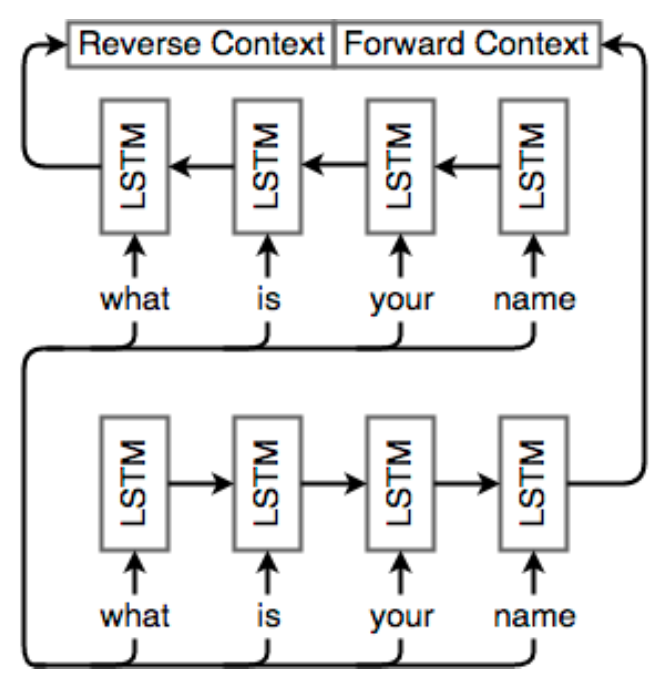
Reference. Stanford CS224n, 2021, Figure: Example of a single-layer bidirectional LSTM encoder network. Note that the input is fed into two different LSTM layers, but in different directions, and the hidden states are concatenated to get the final context vector.

2.5 Multi-layer RNNs

Multi-layer RNNs are also called stacked RNNs.

High-performing RNNs are usually multi-layer (but aren’t as deep as convolutional or feed-forward networks). For example: In a 2017 paper, Britz et al. find that for Neural Machine Translation, 2 to 4 layers is best for the encoder RNN, and 4 layers is best for the decoder RNN. Often 2 layers is a lot better than 1, and 3 might be a little better than 2. Usually, skip-connections/dense-connections are needed to train deeper RNNs(e.g., 8 layers). Transformer-based networks (e.g., BERT) are usually deeper, like 12 or 24 layers.

2.6 Greedy decoding

We saw how to generate (or “decode”) the target sentence by taking argmax on each step of the decoder.

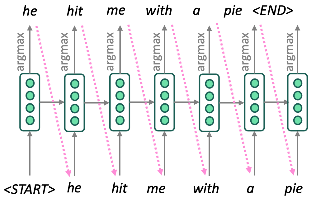
Reference. Stanford CS224n, 2021

Problems with greedy decoding is that greedy decoding has no way to undo decisions.

\[x_t = argmas_{\hat{x_t}}\mathbb{P}(\hat{x}_t \lvert x_1, \dots, x_n)\]

2.7 Exhaustive search decoding

Ideally, we want to find a (length T) translation y that maximizes

\[\begin{aligned} P(y \lvert x) &= P(y_1 \lvert x) P(y_2\lvert y_1, x) P(y_3\lvert y_1, y_2, x) \dots, P(y_T\lvert y_1,\dots, y_{T-1}, x) \\ &= \prod_{t=1}^T P(y_t\lvert y_1, \dots, y_{t-1}, x) \end{aligned}\]

It could try computing all possible sequences y. This means that on each step t of the decoder, we’re tracking Vt possible partial translations, where V is vocab size. But This $O(V^T)$ complexity is far too expensive!

2.8 Ancestral sampling

At time step t, we sample xt based on the conditional probability of the word at step t given the past. In other words,

\[x_t \sim \mathbb{P}(x_t\lvert x_1,\dots, x_n)\]

Theoretically, this technique is efficient and asymptotically exact. However, in practice, it can have low performance and high variance.

2.9 Beam search decoding

Core idea is on each step of decoder, keep track of the k most probable partial translations (which we call hypotheses). k is the beam size (in practice around 5 to 10). A hypothesis $y_1, \dots y_t$ has a score which is its log probability:

\[score(y_1,\dots, y_t) = logP_{LM}(y_1,\dots,y_t \lvert) = \displaystyle\sum_{i=1}^t logP_{LM}(y_i\lvert y_1, \dots, y_{i-1}, x)\]

Scores are all negative, and higher score is better. We search for high -scoring hypotheses, tracking top k on each step. Beam search is not guaranteed to find optimal solution, but much more efficient than Exhaustive search decoding.

Sequence

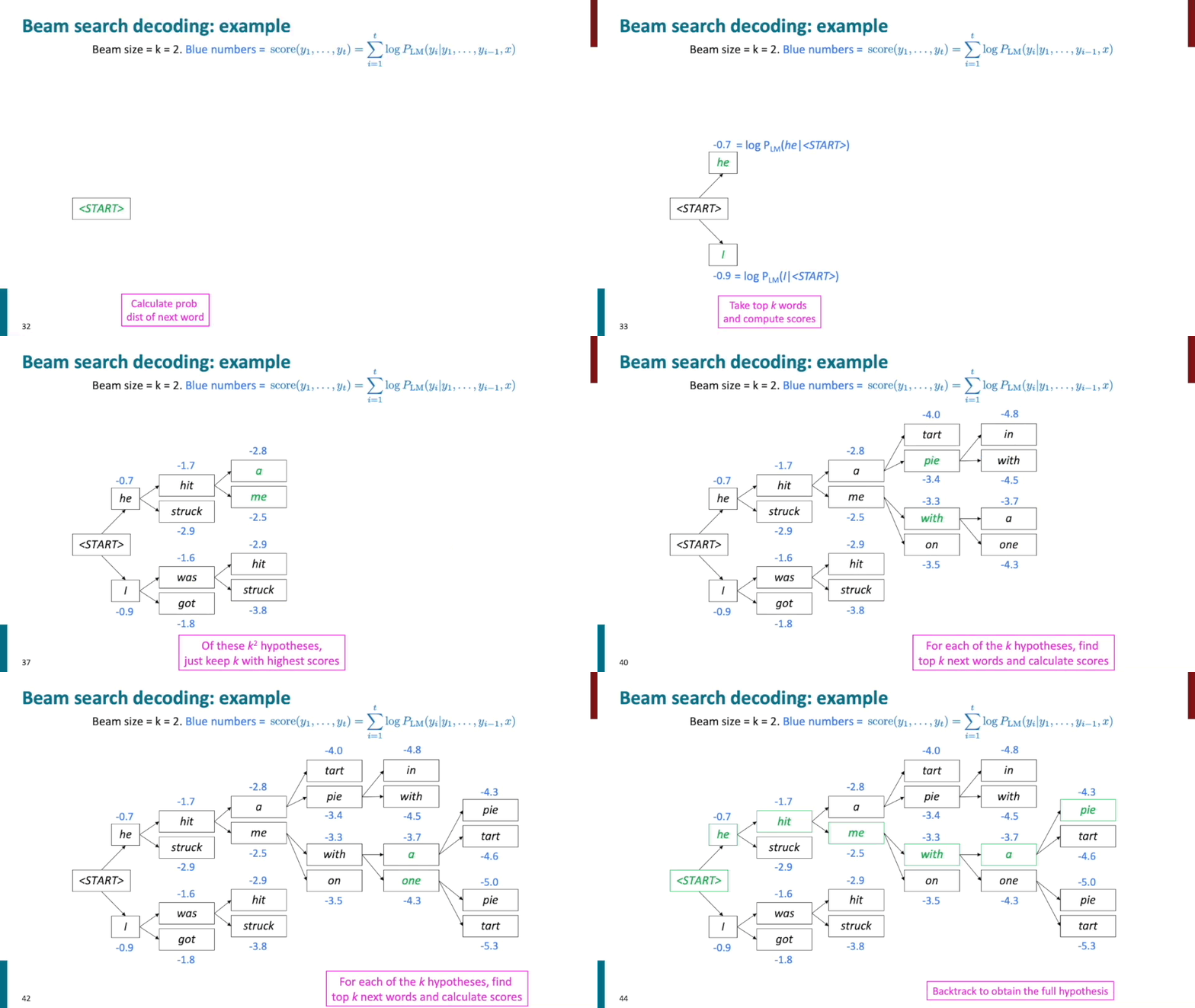
Reference. Stanford CS224n, 2021

In greedy decoding, usually we decode until the model produces an token. In beam search decoding, different hypotheses may produce tokens on different timesteps. When a hypothesis produces , that hypothesis is complete. Place it aside and continue exploring other hypotheses via beam search. Usually we continue beam search until: We reach time step T(where T is some pre-defined cutoff), or We have at least n completed hypotheses(where n is pre-defined cutoff).

Problem is that longer hypotheses have lower scores. So Normalize by length. Use this to select top one instead:

\[\dfrac{1}{t} \displaystyle\sum_{i=1}^t logP_{LM}(y_i\lvert y_1, \dots, y_{i-1}, x)\]

Difference Explanation

the idea is to maintain K candidates at each time step.
\[\mathcal{H}_t = \{(x_1^1, \dots, x_t^1), \dots, (x_1^K, \dots, x_t^K)\}\]
and compute $H_{t+1}$ by expanding Ht and keeping the best K candidates. In other words, we pick the best K sequence in the following set
\[\hat{\mathcal{H}_{t+1}} = \displaystyle\bigcup_{k=1}^K \mathcal{H}_{t+1}^{\hat{k}}\]
where
\[\mathcal{H}_{t+1}^{\hat{k}} = \{(x_1^k, \dots, x_t^k,v_1), \dots, (x_1^k, \dots, x_t^k, v_{\lvert V \lvert})\}\]
As we increase K, we gain precision and we are asymptotically exact. However, the improvement is not monotonic and we canset a K that combines reasonable performance and computational efficiency. For this reason, beam search is the most commonly used technique in NMT.

2.10 Advanteage of NMT

First, Better performance(fluent, use of context, use of phrase similarities). Second, A single neural network is optimized end-to-end. it can be no subcomponents to be individually optimized. Third, Requires much less human engineering effort. It means No feature engineering and Same method for all language pairs. But NMT is less interpretable so it is hard to debug. And NMT is difficult to control. For example it can’t easily specify rules or guidelines for translation.

2.11 How do we evaluate Machine Translation?

Evaluating the quality of machine learning translations has become it own entire research area, with many proposals like TER, METEOR, MaxSim, SEPIA, and RTE-MT. We will focus in these notes on two baseline evaluation methods and BLEU.

$\checkmark$ BLEU (Bilingual Evaluation Understudy)

BLEU compares the machine-written translation to one or several human-written translation(s), and computes a similarity score based on: n-gram precision (usually for 1, 2, 3 and 4-grams) and a penalty for too-short system translations. Its limitation is there are many valid ways to translate a sentence. So a good translation can get a poor BLEU score because it has low n-gram overlap with the human translation.

In 2002, IBM researchers developed the Bilingual Evaluation Understudy (BLEU) that remains, with its many variants to this day, one of the most respected and reliable methods for machine translation.

The BLEU algorithm evaluates the precision score of a candidate machine translation against a reference human translation. The reference human translation is a assumed to be a model example of a translation, and we use n-gram matches as our metric for how similar a candidate translation is to it. Consider a reference sentence A and candidate translation B:

A there are many ways to evaluate the quality of a translation, like comparing the number of n-grams between a candidate transla- tion and reference.
B the quality of a translation is evaluate of n-grams in a reference and with translation.

The BLEU score looks for whether n-grams in the machine translation also appear in the reference translation. Color-coded below are some examples of different size n-grams that are shared between the reference and candidate translation.

The BLEU algorithm identifies all such matches of n-grams above, including the unigram matches, and evaluates the strength of the match with the precision score. The precision score is the fraction of n-grams in the translation that also appear in the reference.

The algorithm also satisfies two other constraints. For each n-gram size, a gram in the reference translation cannot be matched more than once. For example, the unigram “a” appears twice in B but only once in A. This only counts for one match between the sentences. Additionally, we impose a brevity penalty so that very small sentences that would achieve a 1.0 precision (a “perfect” matching) are not considered good translations. For example, the single word “there” would achieve a 1.0 precision match, but it is obviously not a good match.

Let us see how to actually compute the BLEU score. First let k be the maximum n-gram that we want to evaluate our score on. That is, if k = 4, the BLEU score only counts the number of n-grams with length less than or equal to 4, and ignores larger n-grams. Let

\[p_n = \text{# matched n-grams / # n-grams in candidate transition}\]

the precision score for the grams of length n. Finally, let $w_n = 1/2^n$ be a geometric weighting for the precision of the n’th gram. Our brevity penalty is defined as

\[\beta = e^{min(0,1-\dfrac{len_{ref}}{len_{MT}})}\]

where $len_{ref}$ is the length of the reference translation and lenMT is the length of the machine translation.

The BLEU score is then defined as

\[BLEU = \beta\displaystyle\prod_{i=1}^k p_n^{w_n}\]

The BLEU score has been reported to correlate well with human judgment of good translations, and so remains a benchmark for all evaluation metrics following it. However, it does have many limitations. It only works well on the corpus level because any zeros in precision scores will zero the entire BLEU score. Additionally, this BLEU score as presented suffers for only comparing a candidate translation against a single reference, which is surely a noisy representation of the relevant n-grams that need to be matched. Variants of BLEU have modified the algorithm to compare the candidate with multiple reference examples. Additionally, BLEU scores may only be a necessary but not sufficient benchmark to pass for a good machine translation system. Many researchers have optimized BLEU scores until they have begun to approach the same BLEU scores between reference translations, but the true quality remains far below human translations.

2.12 Dealing with the large output vocabulary

Despite the success of modern NMT systems, they have a hard time dealing with large vocabulary size. Specifically, these Seq2Seq models predict the next word in the sequence by computing a target proba- bilistic distribution over the entire vocabulary using softmax. It turns out that softmax can be quite expensive to compute with a large vocabulary and its complexity also scales proportionally to the vocabulary size. We will now examine a number of approaches to address this issue.

$\checkmark \text{ 1.}$ Scaling softmax

A very natural idea is to ask “can we find more efficient ways to compute the target probabilistic distribution?” The answer is Yes! In fact, we’ve already learned two methods that can reduce the complexity of “softmax”, which we’ll present a high-level review below (see details in week 1).

1.1. Noise Contrastive Estimation

The idea of NCE is to approximate “softmax” by randomly sampling K words from negative samples. As a result, we are reducing the computational complexity by a factor of $\frac{\lvert V \lvert}{K}$ , where $\lvert V\lvert$ is the vocabulary size. This method has been proven successful in word2vec. A recent work by Zoph et al.7 applied this technique to learning LSTM language models and they also introduced a trick by using the same samples per mini-batch to make the training GPU-efficient.

1.2. Hierarchical Softmax

Morin et al.8 introduced a binary tree structure to more efficiently compute “softmax”. Each probability in the target distributionis calculated by taking a path down the tree which only takes $O(log\lvert V\lvert)$ steps. Notably, even though Hierarchical Softmax saves computation, it cannot be easily parallelized to run efficiently on GPU. This method is used by Kim et al. 9 to train character-based language models which will be covered in lecture 13(in Standford CS224n).

One limitation for both methods is that they only save computation during training step (when target word is known). At test time, one still has to compute the probability of all words in the vocabulary in order to make predictions.

$\checkmark \text{ 2.}$ Reducing vocabulary

Instead of optimizing “softmax”, one can also try to reduce the effective vocabulary size which will speed up both training and test steps. A naive way of doing this is to simply limit the vocabulary size to a small number and replace words outside the vocabulary with a tag <UNK>. Now, both training and test time can be significantly reduced but this is obviously not ideal because we may generate outputs with lots of <UNK>.

Jean et al. 10 proposed a method to maintain a constant vocabulary size $\lvert V′\lvert$ by partitioning the training data into subsets with $\tau$ unique target words, where $\tau = \lvert V′\lvert$. One subset can be found by sequentially scanning the original data set until $\tau$ unique target words are detected(below Figure). And this process is iterated over the entire data set to produce all mini-batch subsets. In practice, we can achieve about 10x saving with $\lvert V\lvert = 500K$ and $\lvert V′\lvert = 30K, 50K$.

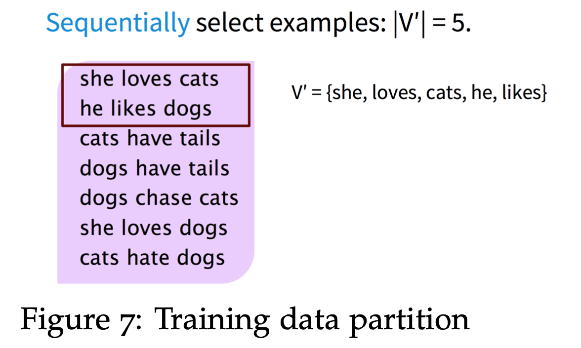
Reference. Stanford CS224n, 2021

This concept is very similar to NCE in that for any given word, the output vocabulary contains the target word and $\lvert V′\lvert − 1$ negative (noise) samples. However, the main difference is that these negative samples are sampled from a biased distribution Q for each subset V’ where

\[Q(y_t) = \begin{cases} \dfrac{1}{\lvert V' \lvert}&, \text{ if } y_t \in \lvert V'\lvert \\ 0 &, \text{ otherwise} \end{cases}\]

At test time, one can similarly predict target word out of a selected subset, called candidate list, of the entire vocabulary. The challenge is that the correct target word is unknown and we have to “guess” what the target word might be. In the paper, the authors proposed to construct a candidate list for each source sentence using K most frequent words (based on unigram probability) and K’ likely target words for each source word in the sentence. In below Figure, an example is shown with K′ = 3 and the candidate list consists of all the words in purple boxes. In practice, one can choose the following values: K = 15k, 30k, 50k and K′ = 10, 20.

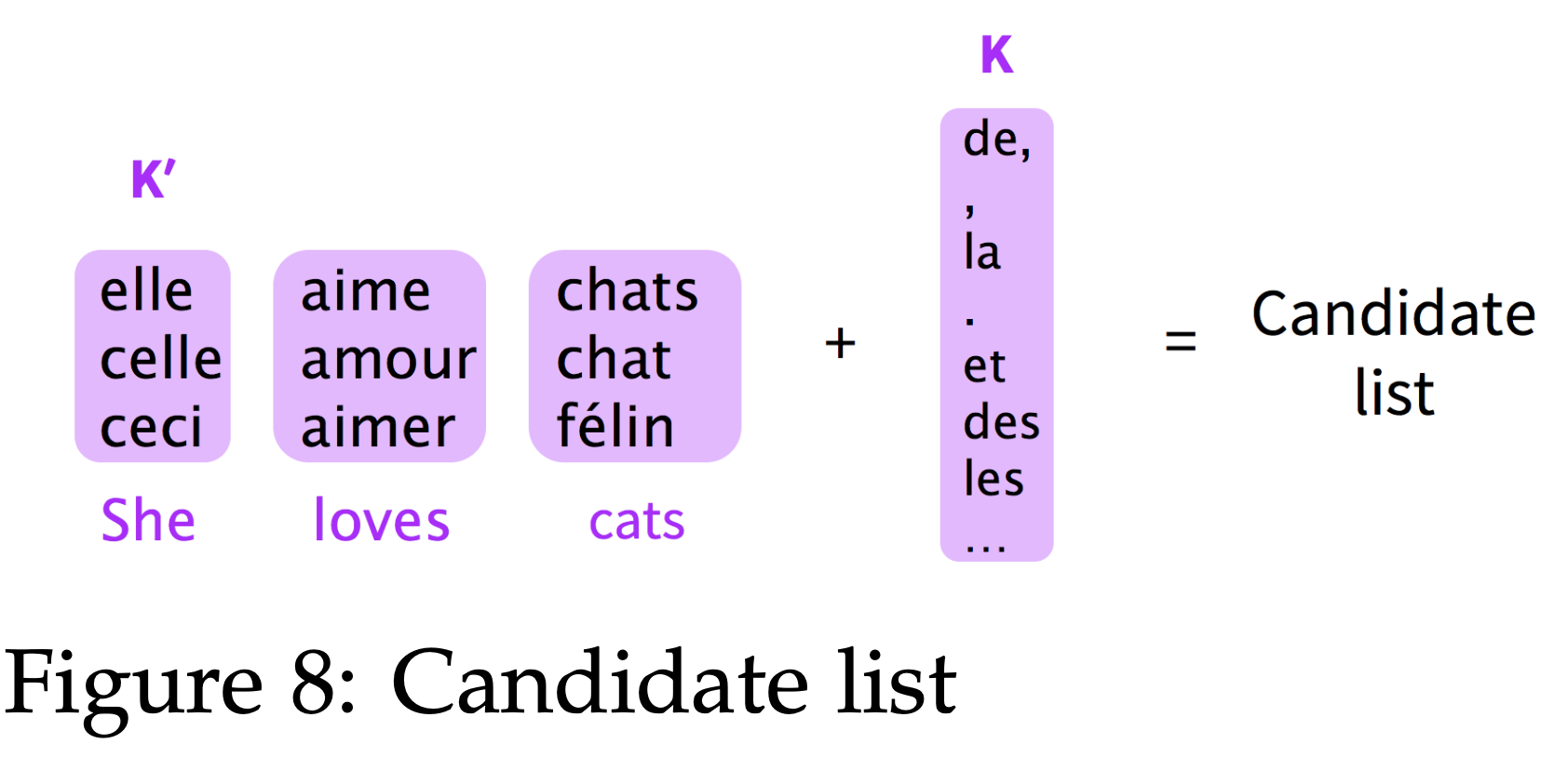
Reference. Stanford CS224n, 2021

$\checkmark \text{ 3.}$ Handling unknown words

When NMT systems use the techniques mentioned above to reduce effective vocabulary size, inevitably, certain words will get mapped to <UNK>. For instance, this could happen when the predicted word, usually rare word, is out of the candidate list or when we encounter unseen words at test time. We need new mechanisms to address the rare and unknown word problems.

One idea introduced by Gulcehre et al. 11 to deal with these problems is to learn to “copy” from source text. The model (below Figure) applies attention distribution $l_t$ to decide where to point in the source text and uses the decoder hidden state St to predict a binary variable $Z_t$ which decides when to copy from source text. The final prediction is either the word $y^w_t$ chosen by softmax over candidate list, as in previous methods, or $y^l_t$ copied from source text depending on the value of $Z_t$. They showed that this method improves performance in tasks like machine translation and text summarization.

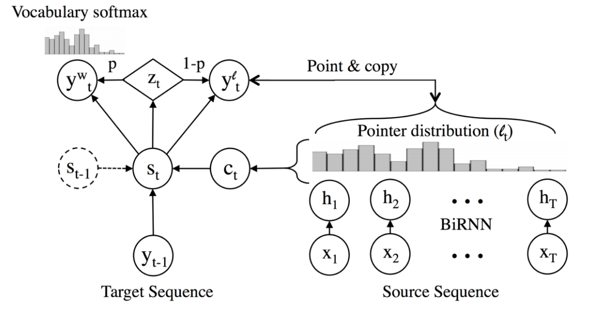
Reference. Stanford CS224n, 2021, Figure: Pointer network Architecture 11 Gulcehre et al. 2016, Pointing the Unknown Words

As one can imagine, there are of course limitations to this method. It is important to point out a comment from Google’s NMT paper 12 on this method, “ this approach is both unreliable at scale — the attention mechanism is unstable when the network is deep — and copying may not always be the best strategy for rare words — sometimes transliteration is more appropriate”.

2.13 Word and character-based models

As discussed in previous section, “copy” mechanisms are still not sufficient in dealing with rare or unknown words. Another direction to address these problems is to operate at sub-word levels. One trend is to use the same seq2seq architecture but operate on a smaller unit — word segmentation, character-based models. Another trend is to embrace hybrid architectures for words and characters.

Word segmentation

Sennrich et al. 13 proposed a method to enable open-vocabulary translation by representing rare and unknown words as a sequence of subword units.

This is achieved by adapting a compression algorithm called Byte Pair Encoding. The essential idea is to start with a vocabulary of characters and keep extending the vocabulary with most frequent n-gram pairs in the data set. For instance, in below figure, our data set contains 4 words with their frequencies on the left, i.e. “low” appears 5 times. Denote ( p, q, f ) as a n-gram pair p, q with frequency f. In this figure, we’ve already selected most frequent n-gram pair (e,s,9) and now we are adding current most frequent n-gram pair (es,t,9). This process is repeated until all n-gram pairs are selected or vocabulary size reaches some threshold.

Reference. Stanford CS224n, 2021, Figure : Byte Pair Encoding

One can choose to either build separate vocabularies for training and test sets or build one vocabulary jointly. After the vocabulary is built, an NMT system with some seq2seq architecture (the paper used Bahdanau et al. 14), can be directly trained on these word segments. Notably, this method won top places in WMT 2016.

Character-based model

Ling et al. 15 proposed a character-based model to enable open vocabulary word representation.For each word w with m characters, instead of storing a word embedding, this model iterates over all characters c1, c2 . . . cm to look up the character embeddings e1, e2 . . . em. These character embeddings are then fed into a bi-LSTM to get the final hidden states hf , hb for forward and backward directions respectively. The final word embedding is computed by an affine transformation of two hidden states:

\[e_w = W_fH_f + W_bH_b + b\]

There are also a family of CNN character-based models which will be covered in lecture 13(in Stanford 224N).

2.14 Hybrid NMT

Luong et al. 16 proposed a Hybrid Word-Character model to deal with unknown words and achieve open-vocabulary NMT. The system translates mostly at word-level and consults the character components for rare words. On a high level, the character-level recurrent neural networks compute source word representations and recover unknown target words when needed. The twofold advantage of such a hybrid approach is that it is much faster and easier to train than character-based ones; at the same time, it never produces unknown words as in the case of word-based models.

Word-based Translation as a Backbone The core of the hybrid NMT is a deep LSTM encoder-decoder that translates at the word level. We maintain a vocabulary of size $\lvert V\lvert$ per language and use <unk> to represent out of vocabulary words.

Source Character-based Representation In regular word-based NMT, a universal embedding for <unk> is used to represent all out-of-vocabulary words. This is problematic because it discards valuable information about the source words. Instead, we learn a deep LSTM model over characters of rare words, and use the final hidden state of the LSTM as the representation for the rare word (below Figure).

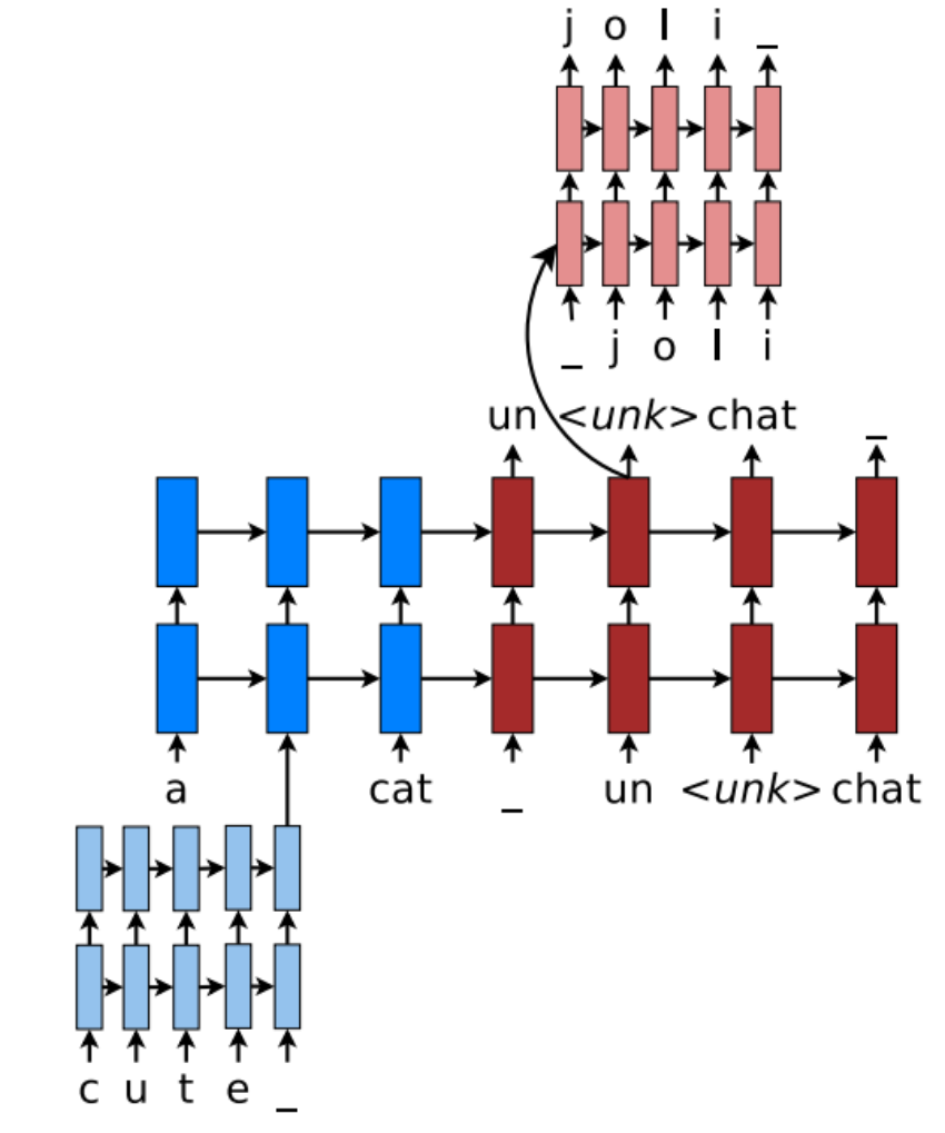
Reference. Stanford CS224n, 2021, Figure: Hybrid NMT

Target Character-level Generation General word-based NMT allows generation of <unk> in the target output. Instead, the goal here is to create a coherent framework that handles an unlimited output vocabulary. The solution is to have a separate deep LSTM that “translates” at the character level given the current word-level state. Note that the current word context is used to initialize the character- level encoder. The system is trained such that whenever the word- level NMT produces an <unk>, the character-level decoder is asked to recover the correct surface form of the unknown target word.

2.15 What is the difficulties about Machine Translation?

Out-of-vocabulary words
Domain mismatch between train and test data
Maintaining context over longer text
Low-resource language pairs
Failures to accurately capture sentence meaning
Pronoun (or zero pronoun) resolution errors
Morphological agreement errors
Using common sense is still hard
NMT picks up biases in training data
Uninterpretable systems do strange things

3. Attention

3.1 Motivation

Sequence-to-sequence: the bottleneck problem, When you hear the sentence “the ball is on the field,” you don’t assign the same importance to all 6 words. You primarily take note of the words “ball,” “on,” and “field,” since those are the words that are most “important” to you. Similarly, Bahdanau et al. noticed the flaw in using the final RNN hidden state as the single “context vector” for sequence-to-sequence models: often, different parts of an input have different levels of significance. Moreover, different parts of the output may even consider different parts of the input “important.” For exam- ple, in translation, the first word of output is usually based on the first few words of the input, but the last word is likely based on the last few words of input.

Attention mechanisms make use of this observation by providing the decoder network with a look at the entire input sequence at every decoding step; the decoder can then decide what input words are important at any point in time. There are many types of encoder mechanisms, but we’ll examine the one introduced by Bahdanau et al.

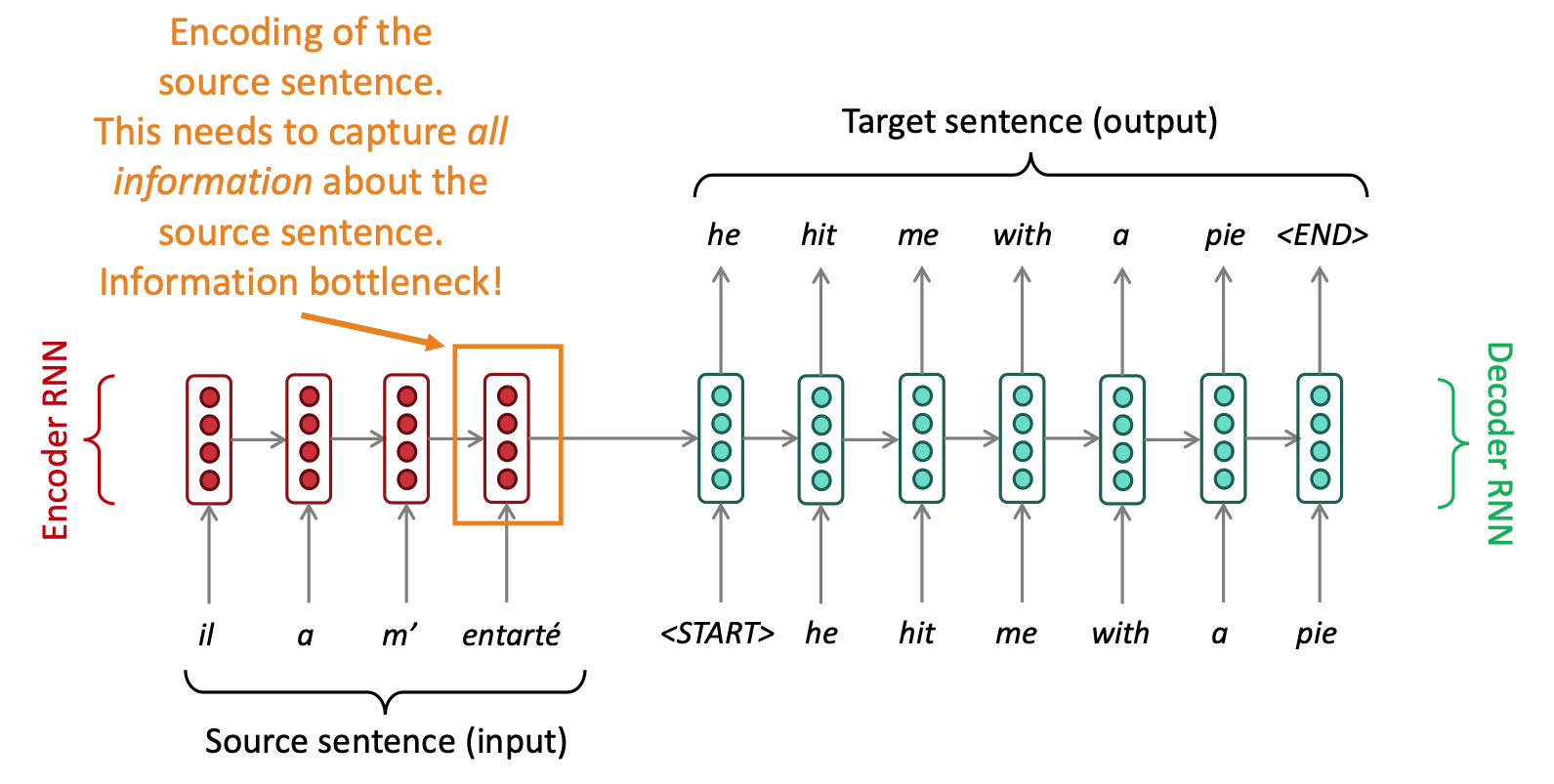
Reference. Stanford CS224n, 2021

Attention provides a solution to the bottleneck problem. On each step of the decoder, use direct connection to the encoder to focus.

3.2 Sequence

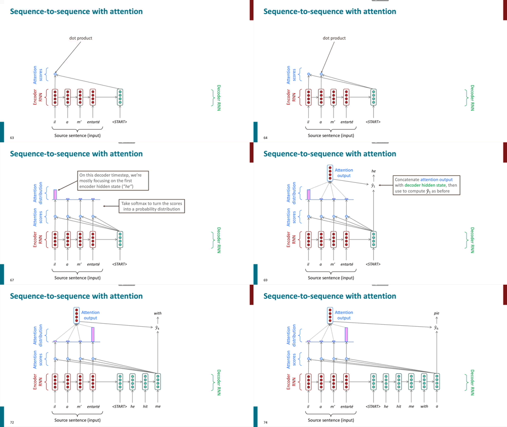
Reference. Stanford CS224n, 2021

In equation,

We have encoder hidden states $h_1,…,h_N \in \mathbb{R}^h$
On timestep t, we have decoder hidden state $s_t \in \mathbb{R}^h$
We get the attention scores for this step:
\[e^t = [s_t^T h_1,...,s_t^Th_N] \in \mathbb{R}^N\]
We take softmax to get the attention distribution $\alpha^t$ for this step (this is a probability distribution and sums to 1)
\[\alpha^t = softmax(e^t) \in \mathbb{R}^N\]
We use $\alpha^t$ to take a weighted sum of the encoder hidden states to get the attention output $a_t$
\[a_t = \displaystyle\sum_{i=1}^N \alpha_i^th_i \in \mathbb{R}^h\]
Finally we concatenate the attention output with the decoder hidden state $s_t$ and proceed as in the non-attention seq2seq model
\[[a_t;s_t] \in \mathbb{R}^{2h}\]

Results about “Attention is great”

Attention significantly improves NMT performance
Attention solves the bottleneck problem
Attention helps with vanishing gradient problem
Attention provides some interpretability
By inspecting attention distribution, we can see what the decoder was focusing on
- We get (soft) alignment for free!
- This is cool because we never explicitly trained an alignment system.
- The network just learned alignment by itself

More general definition of attention:

Given a set of vector values, and a vector query, attention is a technique to compute a weighted sum of the values, dependent on the query.

We sometimes say that the query attends to the values. For example, in the seq2seq + attention model, each decoder hidden state (query) attends to all the encoder hidden states (values).

Intuition

The weighted sum is a selective summary of the information contained in the values, where the query determines which values to focus on.
Attention is a way to obtain a fixed-size representation of an arbitrary set of representations (the values), dependent on some other representation (the query).

3.3 Several attention variants

We have some values $h_1,…,h_N \in \mathbb{R}^{d_1}$and a query $s \in \mathbb{R}^{d_2}$

Attention always involves:

Computing the attention scores $e \in \mathbb{R}^N$ : There are multiple ways to do this
Taking softmax to get attention distribution ⍺:

\[\alpha = softmax(e) \in \mathbb{R}^N\]

Using attention distribution to take weighted sum of values:

\[a = \displaystyle\sum_{i=1}^N \alpha_i h_i \in \mathbb{R}^{d_1}\]

thus obtaining the attention output $a$ (sometimes called the context vector)

3.4 Attention variants

There are several ways you can compute $e \in \mathbb{R}^N$ from $h_1,…,h_N \in \mathbb{R}^{d_1}$ and $s \in \mathbb{R}^{d_2}$

Basic dot-product attention: $e_i=s^Th_i \in \mathbb{R}$
- Note: this assumes $d_1=d_2$
- This is the version we saw earlier
Multiplicative attention: $e_i=s^TWh_i \in \mathbb{R}$
- Where $W \in \mathbb{R}^{d_2 \times d_1}$ is a weight matrix
Additive attention: $e_i=v^Ttanh(W_1h_i + W_2s) \in \mathbb{R}$
- Where $W \in \mathbb{R}^{d_3 \times d_1}$, $W_2 \in \mathbb{R}^{d_3 \times d_2}$are weight matrices and is a weight vector.
- $d_3$ (the attention dimensionality) is a hyperparameter - More information
- “Deep Learning for NLP Best Practices”, Ruder, 2017.
- “Massive Exploration of Neural Machine Translation Architectures”, Britz et al, 2017

3.5 Attention Models

$\checkmark$ Bahdanau et al. NMT model

Remember that our seq2seq model is made of two parts, an encoder that encodes the input sentence, and a decoder that leverages the information extracted by the decoder to produce the translated sentence. Basically, our input is a sequence of words x1, . . . , xn that we want to translate, and our target sentence is a sequence of words y1,…,ym.

Encoder

Let (h1, . . . , hn) be the hidden vectors representing the input sentence. These vectors are the output of a bi-LSTM for instance, and capture contextual representation of each word in the sentence.
Decoder

We want to compute the hidden states si of the decoder using a recursive formula of the form
\[s_i = f(s_{i−1},y_{i−1},c_i)\]
where $s_{i−1}$ is the previous hidden vector, $y_{i−1}$is the generated word at the previous step, and ci is a context vector that capture the context from the original sentence that is relevant to the time step i of the decoder.

The context vector ci captures relevant information for the i-th decoding time step (unlike the standard Seq2Seq in which there’s only one context vector). For each hidden vector from the original sentence hj, compute a score
\[e_{i,j} = a(s_{i−1}, h_j)\]
where a is any function with values in R, for instance a single layer fully-connected neural network. Then, we end up with a sequence of scalar values $e_{i,1}, . . . , e_{i,n}$. Normalize these scores into a vector $\alpha_i = (\alpha_{i,1}, . . . , \alpha_{i,n})$, using a softmax layer(called the attention vector).
\[\alpha_{i,j} = \dfrac{exp(e_{i,j})}{\displaystyle\sum_{j=1}^n\alpha_{i,j}h_j}\]
Then, compute the context vector ci as the weighted average of the hidden vectors from the original sentence
\[c_i = \displaystyle\sum_{j=1}^n \alpha_{i,j}h_j\]
Intuitively, this vector captures the relevant contextual information from the original sentence for the i-th step of the decoder.

$\checkmark$ Huong et al. NMT model

We present a variant of this first model, with two different mecha- nisms of attention, from Luong et al.

Global attention We run our vanilla Seq2Seq NMT. We call the hidden states given by the encoder $h_1, . . . , h_n$, and the hidden states of the decoder $\bar h_1 , . . . , \bar h_n$ . Now, for each $\bar h_i$ , we compute an attention vector over the encoder hidden. We can use one of the following scoring functions:

\[\text{score}(h_i, \bar h_j) = \begin{cases} h_i^T\bar h_j \\ h_i^T W \bar h_j & \in \mathbb{R} \\ W[h_i, \bar h_j] \\ \end{cases}\]

Now that we have a vector of scores, we can compute a context vector in the same way as Bahdanau et al. First, we normalize the scores via a softmax layer to obtain a vector $\alpha_i =(\alpha_{i,1},…,\alpha_{i,n})$, where

\[\alpha_{i, j} = \dfrac{\text{exp}(\text{score}(h_j, \bar h_i))}{\sum_{k=1}^n \text{exp}(\text{score}(h_k, \bar h_i))} \\ c_i = \displaystyle\sum_{j=1}^n \alpha_{i, j}h_j\]

and we can use the context vector and the hidden state to compute a new vector for the i-th time step of the decoder

\[\tilde{h_i} = f([\bar h_i, c_i])\]

The final step is to use the $\tilde h_i$ to make the final prediction of the decoder. To address the issue of coverage, Luong et al. also usean input-feeding approach. The attentional vectors $\tilde h_i$ are fed as input to the decoder, instead of the final prediction. This is similar to Bahdanau et al., who use the context vectors to compute the hidden vectors of the decoder.

Local attention the model predicts an aligned position in the input sequence. Then, it computes a context vector using a window centered on this position. The computational cost of this attention step is constant and does not explode with the length of the sentence.

The main takeaway of this discussion is to show that they are lots of ways of doing attention.

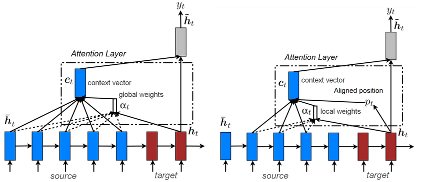
Reference. Stanford CS224n, 2021, Notes on Deep Learning for NLP, Antoine J.-P. Tixier

$\checkmark$ Google’s new NMT

As a brief aside, Google recently made a major breakthrough for NMT via their own translation system. Rather than maintain a full Seq2Seq model for every pair of language that they support – each of which would have to be trained individually, which is a tremendous feat in terms of both data and compute time required – they built a single system that can translate between any two languages. This is a Seq2Seq model that accepts as input a sequence of words and a token specifying what language to translate into. The model uses shared parameters to translate into any target language.

The new multilingual model not only improved their translation performance, it also enabled “zero-shot translation,” in which we can translate between two languages for which we have no translation training data. For instance, if we only had examples of Japanese-English translations and Korean-English translations, Google’s team found that the multilingual NMT system trained on this data could actually generate reasonable Japanese-Korean translations. The powerful implication of this finding is that part of the decoding process is not language-specific, and the model is in fact maintaining an internal representation of the input/output sentences independent of the actual languages involved.

More advanced papers using attention

Show, Attend and Tell: Neural Image Caption Generation with Visual Attention by Kelvin Xu, Jimmy Lei Ba,Ryan Kiros, Kyunghyun Cho, Aaron Courville, Ruslan Salakhutdinov, Richard S. Zemel and Yoshua Bengio. This paper learns words/image alignment.
Modeling Coverage for Neural Machine Translation by Zhaopeng Tu, Zhengdong Lu, Yang Liu, Xiaohua Liu and Hang Li. Their model uses a coverage vector that takes into account the attention history to help future attention.
Incorporating Structural Alignment Biases into an Attentional Neural Translation Model by Cohn, Hoang, Vymolova, Yao, Dyer, Haffari. This paper improves the attention by incorporating other traditional linguistic ideas.

PREVIOUSW3 How to struct the Dependency Parsing and the Problem solved by RNN, Bi-RNN, GRU, LTSM?

NEXTW5 Self-Attention and Transformers