All contents is arranged from CS224N contents. Please see the details to the CS224N!
1. Language Model
Language Modeling is the task of predicting what word comes next.
the students opened their [——] → books? laptops? exams? minds?
A system that does this is called a Language Model. More formally: given a sequence of words $x^{(1)}, x^{(2)}, \dots, x^{(t)}$, compute the probability distribution of the next word $x^{(t+1)}$:
\[P(x^{(t+1)}\lvert x^{(t)},\dots,x^{(1)})\]where $x^{(t+1)}$can be any word in the vocabulary $V = {w_1,\dots,w_{\lvert V\lvert}}$
“Assigns probability to a piece of text”, For example, if we have some text $x^{(1)}, …, x^{(t)}$, then the probability of this text (according to the Language Model) is:
\[\begin{aligned} P(x^{(1)},\dots,x^{(T)}) &= P(x^{(1)})\times P(x^{(2)}\lvert x^{(1)}\times \cdots \times P(x^{(T)}\lvert x^{(T-1)},\dots,x^{(1)})\\ &= \displaystyle\prod_{t=1}^T P(x^{(t)}\lvert x^{(t-1)},\dots,x^{(1)}) \end{aligned}\]1.1 n-gram Language Model
$\checkmark$ Idea
-
the students opened their ____
-
Question: How to learn a Language Model?
-
Answer (pre-Deep Learning): learn an n-gram Language Model
-
Definition: A ngram is a chunk of n consecutive words.
- unigrams: “the”, “students”, “opened”, ”their”
- bigrams: “the students”, “students opened”, “opened their”
- trigrams: “the students opened”, “students opened their”
- 4-grams: “the students opened their”
-
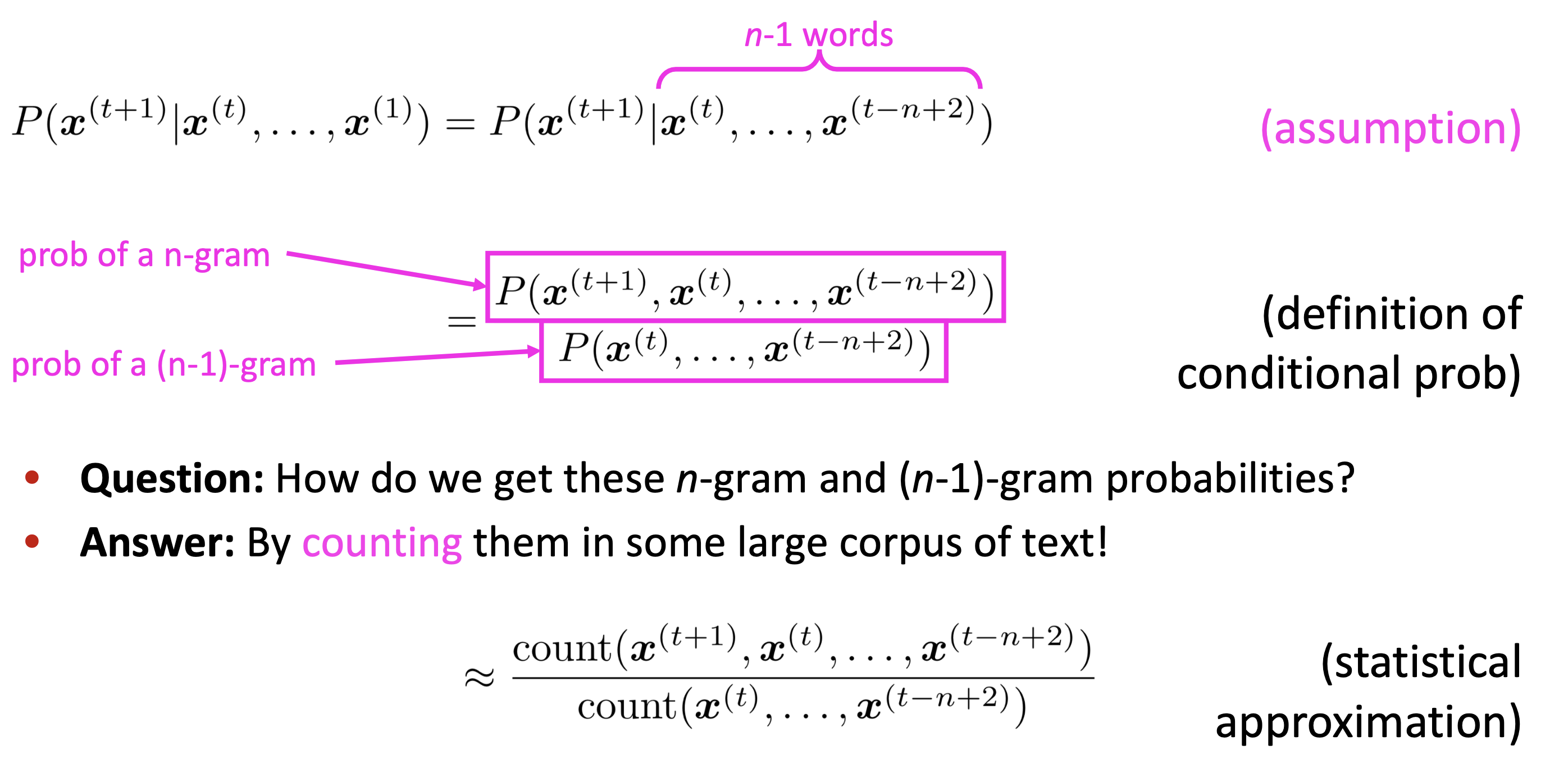
Idea: Collect statistics about how frequent different n-grams are and use these to predict next word.
First we make a Markov assumption: $x^{(t+1)}$ depends only on the preceding n-1 words
Reference. Stanford CS224n, 2021
-
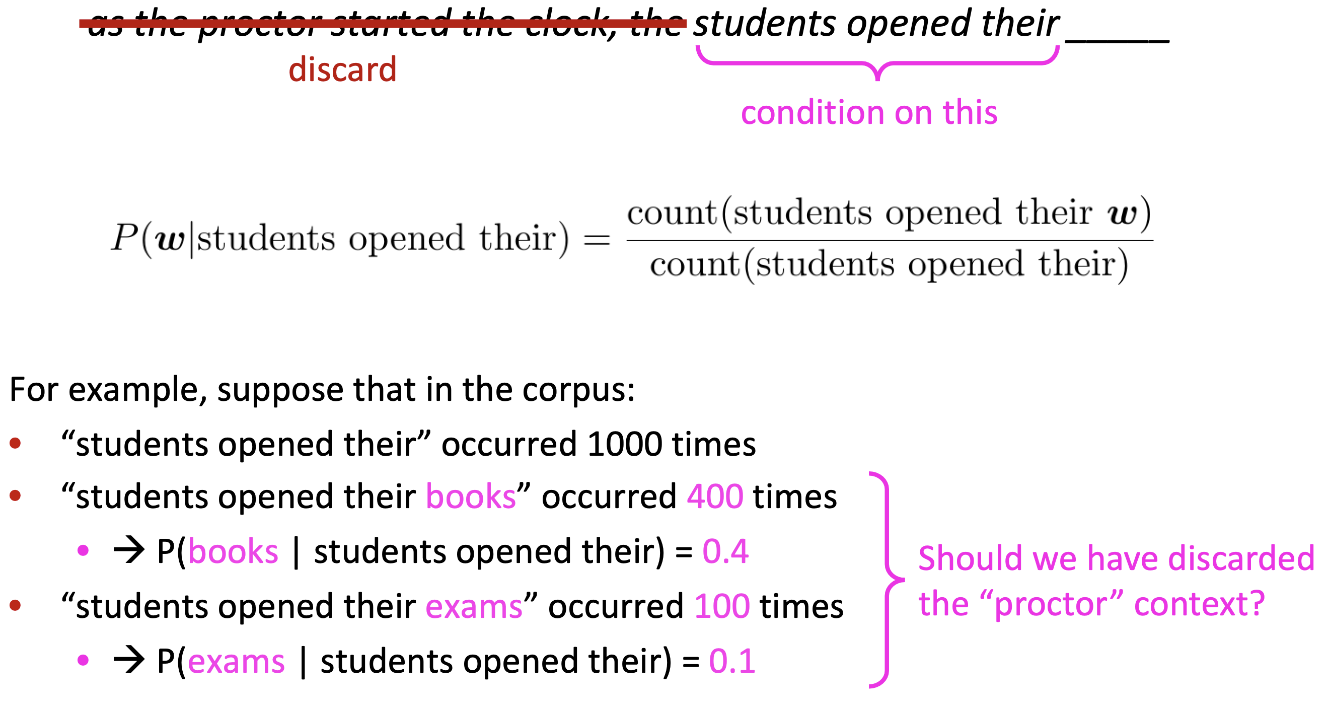
$\checkmark$ Example Suppose we are learning a 4-gram Language Model
Reference. Stanford CS224n, 2021
1.2 Problem
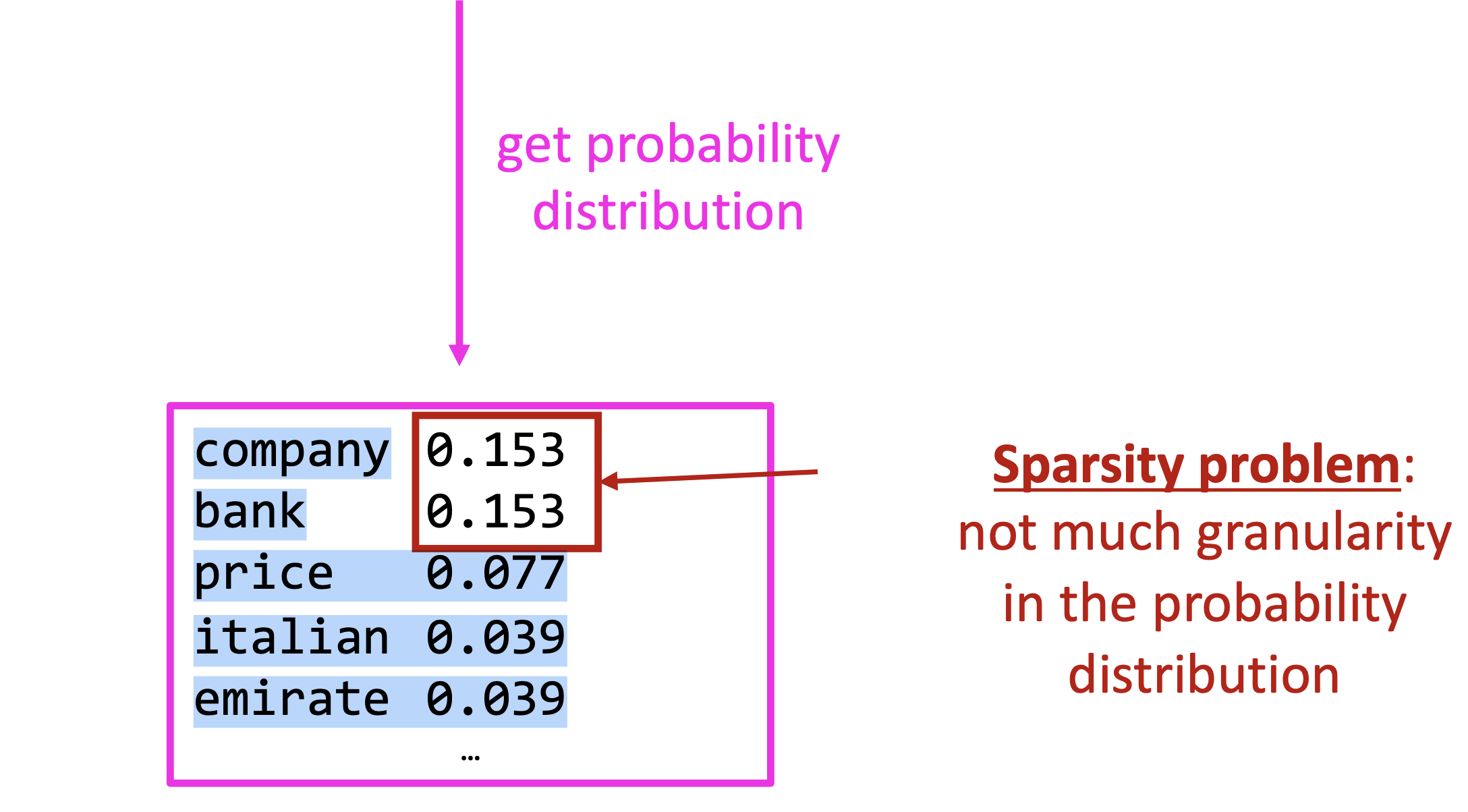
$\checkmark$ Sparsity Problem
Reference. Stanford CS224n, 2021
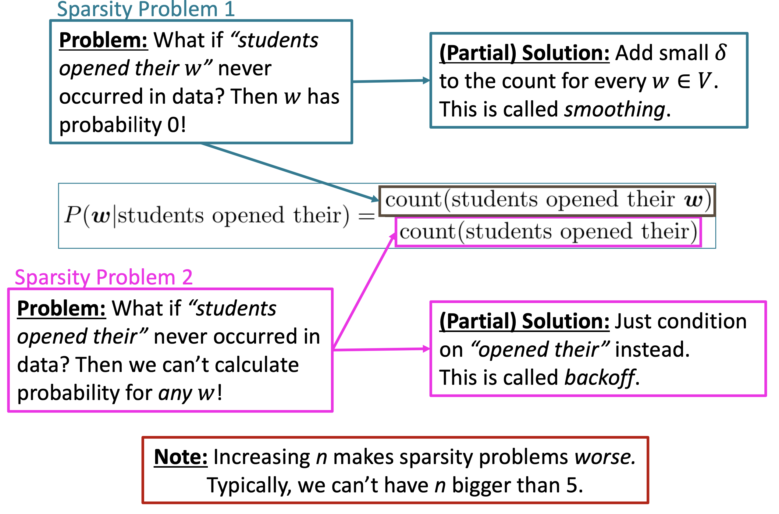
Sparsity problems with these models arise due to two issues.
\[p(w_3\lvert w_1,w_2) = \dfrac{count(w_1,w_2,w_3)}{count(w_1,w_2)}\]Firstly, note the numerator of above Equation. If $w_1$, $w_2$ and $w_3$ never appear together in the corpus, the probability of $w_3$ is 0. To solve this, a small $\delta$ could be added to the count for each word in the vocabulary. This is called smoothing.
Secondly, consider the denominator of Equation 3. If $w_1$ and $w_2$ never occurred together in the corpus, then no probability can be calculated for $w_3$. To solve this, we could condition on $w_2$ alone. This is called backoff.
Increasing $n$ makes sparsity problems worse. Typically, $n \geq 5$
$\checkmark$ Storage Problem
Reference. Stanford CS224n, 2021
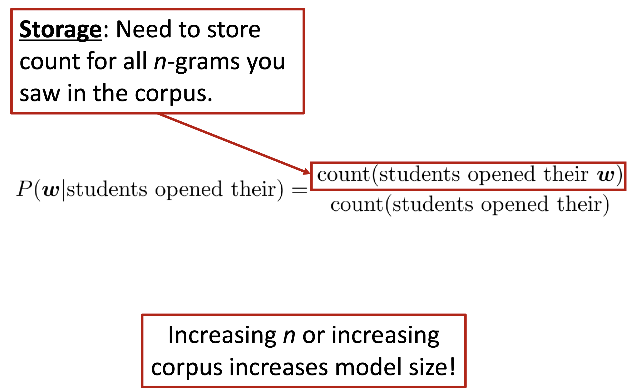
We know that we need to store the count for all n-grams we saw in the corpus. As n increases (or the corpus size increases), the model size increases as well.
$\checkmark$ In Practice
You can build a simple trigram Language Model over a1.7 million word corpus (Reuters- Business and financial news) in a few seconds on your laptop*
- today the ____
Reference. Stanford CS224n, 2021
You can also use a Language Model to generate text

Reference. Stanford CS224n, 2021
$\rightarrow$ Result: today the price of gold per ton , while production of shoe lasts and shoe industry , the bank intervened just after it considered and rejected an imf demand to rebuild depleted european stocks , sept 30 end primary 76 cts a share .
$\rightarrow$ This result is surprisingly grammatical! but incoherent. We need to consider more than three words at a time if we want to model language well. But increasing $n$ worsens sparsity problem, and increases model size…
1.3 Window-based Neural Language Model and RNN
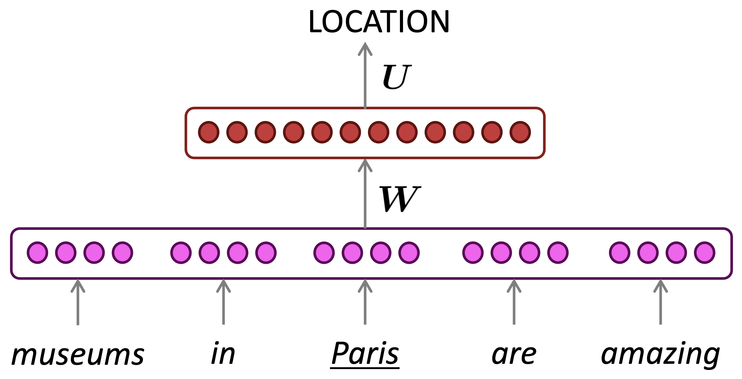
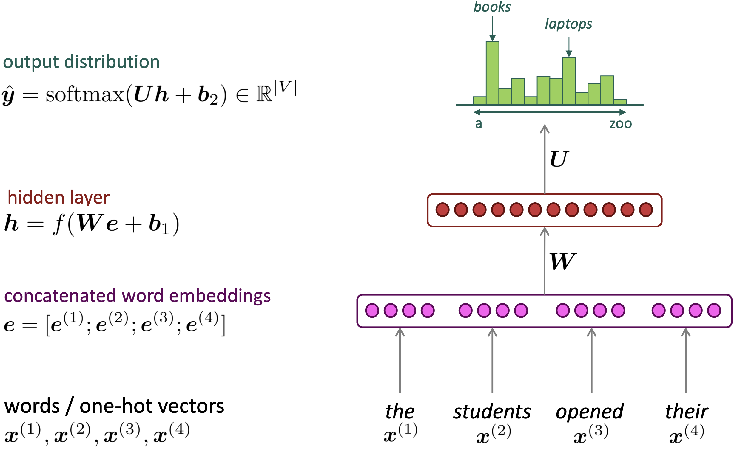
$\checkmark$ A fixed-window neural Language Model
We saw this applied to Named Entity Recognition in Week 2:
Reference. Stanford CS224n, 2021
-
Example

Reference. Stanford CS224n, 2021
-
Structure
Reference. Stanford CS224n, 2021
- Reference. Y. Bengio, et al. (2000/2003): A Neural Probabilistic Language Model
- Improvement over n-gram LM
- No sparsity problem
- Don’t need to store all observed n-grams
- Problems
- Fixed window is too small
- Enlarging window enlarges 𝑊
- Window can never be large enough
- $x^{(1)}$ and $x^{(2)}$ are multiplied by completely different weights in 𝑊. No symmetry in how the inputs are processed.
$\rightarrow$ We need a neural architecture that can process any length input
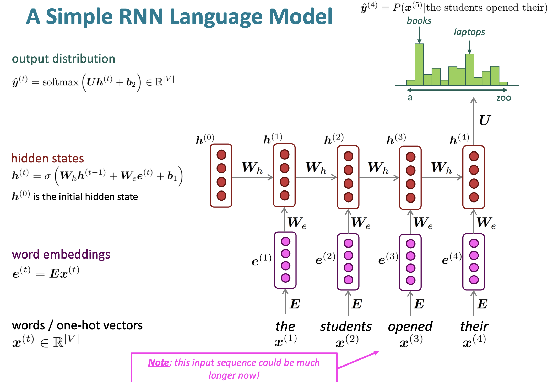
$\checkmark$ Recurrent Neural Networks(RNN)
-
Core idea: Apply the same weights $W$ repeatedly!
-
A Simple RNN Language Model
Reference. Stanford CS224n, 2021
- Advantages
- Can process any length input
- Computation for step t can (in theory) use information from many steps back
- Model size doesn’t increase for longer input context
- Same weights applied on every timestep, so there is symmetry in how inputs are processed.
- Disadvantages
- Recurrent computation is slow
- In practice, difficult to access information from many steps back
- Training Method
- Get a big corpus of text which is a sequence of words $x^{(1)},\dots,x^{(T)}$
- Feed into RNN-LN; compute output distribution $\hat y^{(t)}$ for every step t
- i.e. predict probability dict of every word, given word so far.
-
Loss function on step t is cross-entropy between predicted probability distribution $\hat y^{(t)}$, and the tru next word $y^{(t)}$(one-hot for $x^{(t+1)}$:
\[J^{(t)}(\theta) = CE(y^{(t)}, \hat{y}^{(t)}) = - \displaystyle\sum_{w\in V} y_w^{(t)}log\hat{y}_w^{(t)} = -log\hat{y}_{x_{t+1}}^{(t)}\] -
Average this to get overall loss for entire training set:
\[J(\theta) = \dfrac{1}{T} \displaystyle\sum_{t=1}^T J^{(t)}(\theta) = \dfrac{1}{T} \displaystyle\sum_{t=1}^T -log\hat{y}_{x_{t+1}}^{(t)}\]
-
Total Sequence
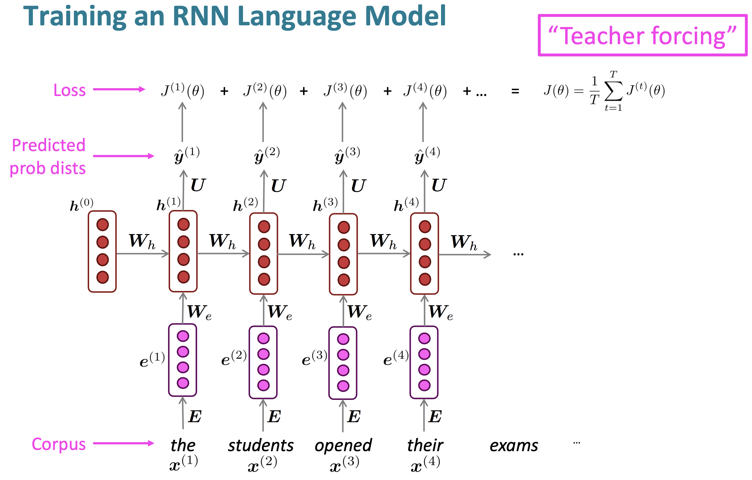
Reference. Stanford CS224n, 2021
However, Computing loss and gradients across entire corpus is too expensive.
\[J(\theta)=\dfrac{1}{T}\displaystyle\sum_{t=1}^T J^{(t)}(\theta)\]In practice, consider $x^{(1)},\dots,x^{(T)}$ as a sentence (or a document). Stochastic Gradient Descent allows us to compute loss and gradients for small chunk of data, and update. Compute loss for a sentence (actually, a batch of sentences), compute gradients and update weights. Repeat.
- Advantages
-
Backpropagation for RNNs
Q. What’s the derivative of $J^{(t)}(\theta)$ w.r.t. the repeated weight matrix $W_h$?
A. $\dfrac{\partial J^{(t)}}{\partial W_h}=\displaystyle\sum_{i=1}^t \dfrac{\partial J^{(t)}}{\partial W_h}\lvert _{(i)}$
“The gradient w.r.t. a repeated weight is the sum of the gradientw.r.t. each time it appears”
- Why? Multivariable Chain Rule
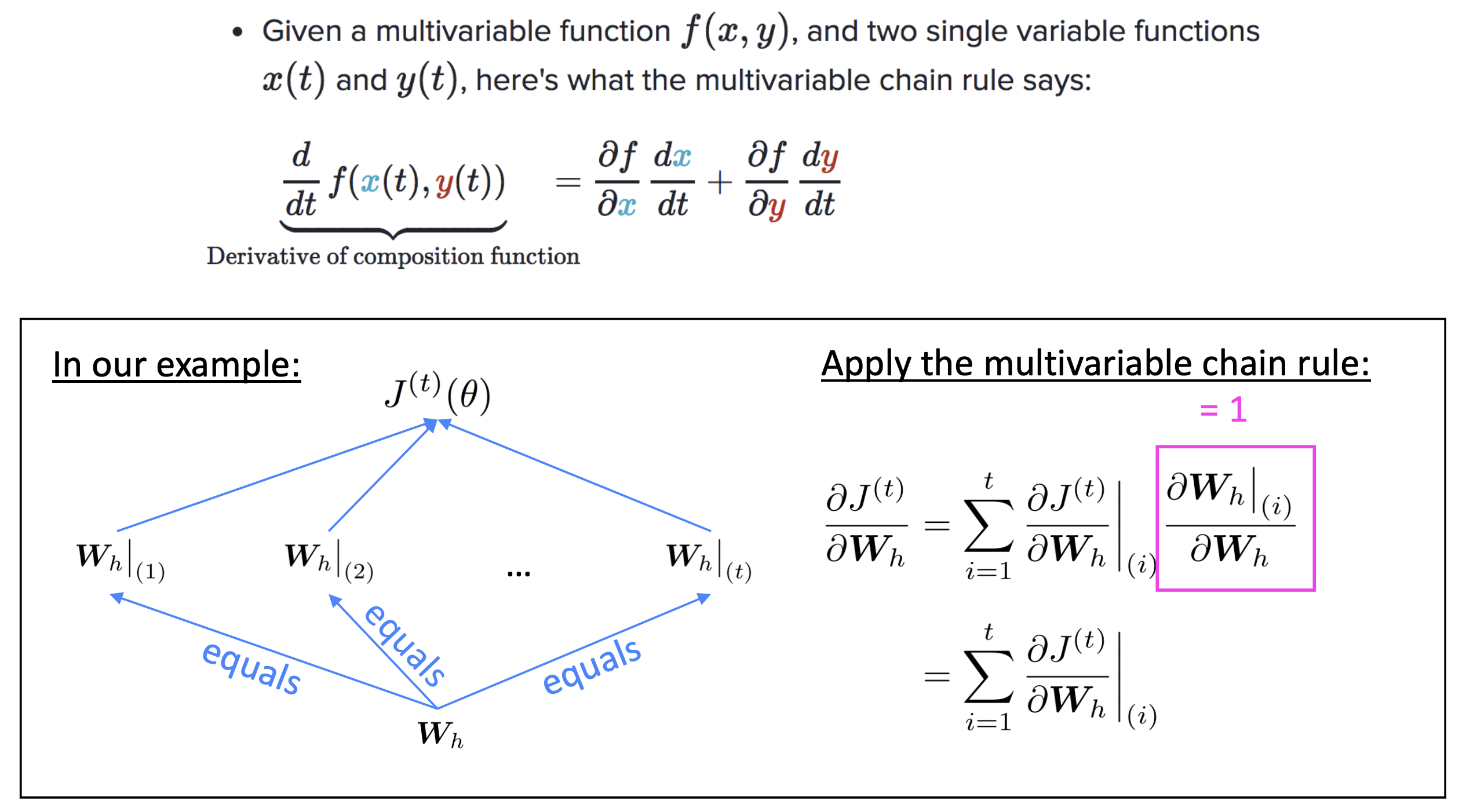
Reference. Stanford CS224n, 2021
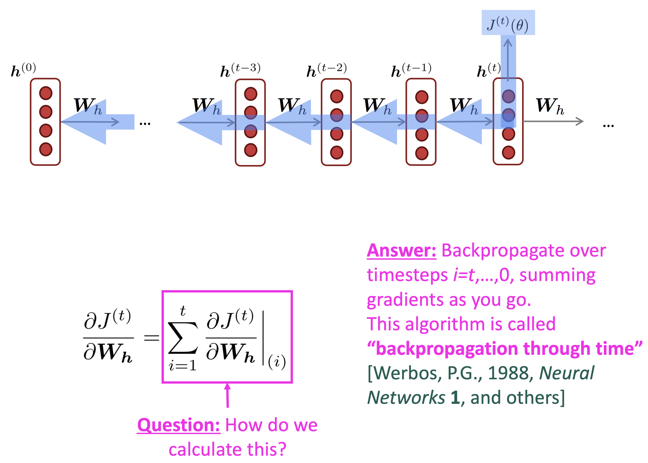
Reference. Stanford CS224n, 2021
Just like a n-gram Language Model, you can use a RNN Language Model to generate text by repeated sampling. Sampled output becomes next step’s input.
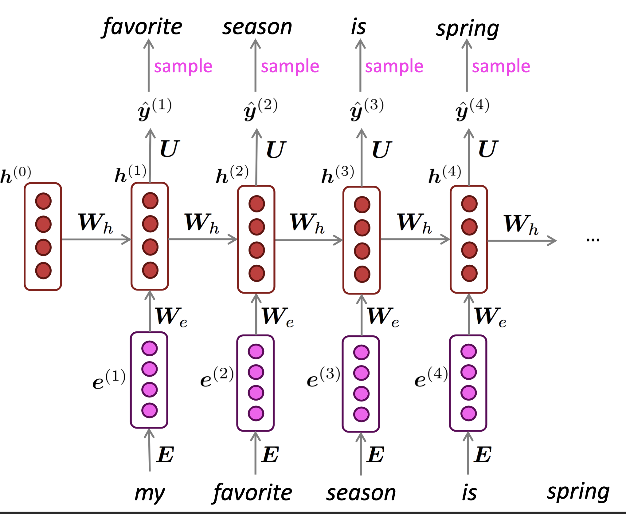
Reference. Stanford CS224n, 2021
$\checkmark$ Evaluating Language Models
“Perplexity”, the standard evaluation metric

Reference. Stanford CS224n, 2021
This is equal to the exponential of the cross-entropy loss $J(\theta)$:
\[= \displaystyle\prod_{t=1}^T\big{(}\dfrac{1}{\hat{y}_{x_{t+1}^{(t)}}}\big{)}^{1/T} = \text{exp}\big{(}\dfrac{1}{T} \displaystyle\sum_{t=1}^T -log\hat{y}_{x_{t+1}}^{(t)} \big{)} = \text{exp}(J(\theta))\]$\rightarrow$ Lower perplexity is better !
2. Exploding, and vanishing gradients
2.1 Vanishing gradients
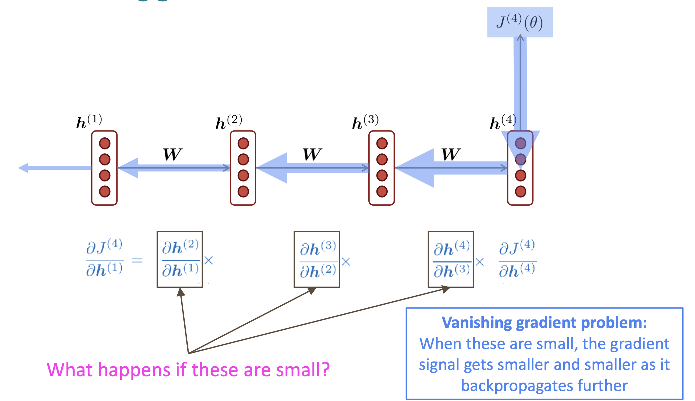
Reference. Stanford CS224n, 2021
-
Linear case
Recall: $h^{(t)}=\sigma(W_hh^{(t-1)}+W_x x^{(t)}+b_1)$
What if $\sigma$ were the identity function(Linear case), $\sigma(x) = x ?$
\[\begin{aligned} \dfrac{\partial h^{(t)}}{\partial h^{(t-1)}} &= diag(\sigma'(W_h h^{(t-1)}+W_x x^{(t)} + b_1))W_h \text{ chain rule} \\ &= IW_h = W_h \end{aligned}\]Consider the gradient of the loss $J^{(i)}(\theta)$ on step i, with repect to the hidden state $h^{(j)}$ on some previous step j. Let $l=i-j$
\[\begin{aligned} \dfrac{\partial J^{(i)}(\theta)}{\partial h^{(j)}} &= \dfrac{\partial J^{(i)}(\theta)}{\partial h^{(j)}} \displaystyle\prod_{j<t \leq i} \dfrac{\partial h^{(t)}}{\partial h^{(t-1)}} \text{ (chain rule)}\\ &= \dfrac{\partial J^{(i)}(\theta)}{\partial h^{(j)}} \displaystyle\prod_{j<t \leq i}W_h = \dfrac{\partial J^{(i)}(\theta)}{\partial h^{(i)}} W_h^l , (\text{value of }\dfrac{\partial h^{(t)}}{\partial h^{(t-1)}}) \end{aligned}\]If $W_h$ is “small”, then this term gets exponentially problematic as $l$becomes large.
-
What’s wrong with $W_h^l$ ?
Consider if the eigenvalues of $W_h$ are all less than 1 (sufficient but not necessary):
\[\lambda_1, \lambda_2, \dots, \lambda_n < 1 \\ q_1, q_2, \dots, q_n \text{ (eigenvectors)}\]We can write $\dfrac{\partial J^{(i)}(\theta)}{h^{(i)}}W_h^l$ using the eigenvectors of $W_h$ as a basis.
-
Proof
\[x_t = W_h\sigma(x_{t-1})+W_{in}u_t+b \text{ (1)}\]Let us consider the term $g_k^T = \dfrac{\partial \varepsilon_t}{\partial x_t} \dfrac{\partial x_t}{\partial x_k} \dfrac{\partial^+ x_k}{\partial \theta}$ for the linear version of the parameterization in equation (1) (i.e. set $\sigma$ to the identity function) and assume t goes to infinity and $l = t - k$. We have that:
\[\dfrac{\partial x_t}{\partial x_k}=(W_{h}^T)^l\]By employing a generic power iteration method based proof we can show that, given certain conditions, $\dfrac{\partial \varepsilon_t}{\partial x_t}(W_{h}^T)^l$ grows exponentially.
Proof Let $W_h^l$ have the eigenvalues $\lambda_1, .., \lambda_n$ with $\lvert\lambda_1\lvert > \lvert\lambda_2\lvert > .. > \lvert\lambda_n\lvert$ and the corresponding eigenvectors $q_1, q_2, .., q_n$ which form a vector basis. We can now write the row vector $\dfrac{\partial \varepsilon_t}{\partial x_t}$into this basis:
\[$\dfrac{\partial \varepsilon_t}{\partial x_t} = \sum_{i=1}^N c_iq_i^T$\]If j is such that $c_j \not= 0$ and any $j’ < j, c_{j’}=0$, using the fact that
$q_i^T(W_h^T)^l=\lambda_i^lq_I^T$ we have that
$\dfrac{\partial \varepsilon_t}{\partial x_t} \dfrac{\partial x_t}{\partial x_k}= c_j\lambda_j^lq_j^T+\lambda_j^l\displaystyle\sum_{i=j+1}^n c_i\dfrac{\lambda_i^l}{\lambda_j^l}q_i^T \approx c_j\lambda_j^lq_j^T$
We used the fact that $\lvert\lambda_i/\lambda_k\lvert<1$ for $i>j$, wihch means that $lim_{l \rightarrow \infty}\lvert\lambda_i/\lambda_k\lvert^l=0$. If $\lvert\lambda\lvert > 1$, it follows that $\dfrac{\partial x_t}{\partial x_k}$ grows exponetially fast with $l$, and it does so along the dircetion $q_j$.
The proof assumes $W_h$is diagonalizable for simplicity, though using the Jordan normal form of $W_h$ one can extend this proof by considering not just the eigenvector of largest eigenvalue but the whole subspace spanned by the eigenvectors sharing the same (largest) eigenvalue.
This result provides a necessary condition for gradients to grow, namely that the spectral radius (the absolute value of the largest eigenvalue) of $W_h$ must be larger than 1.
→ Then smaller than 1 = gradient $\approx$ 0
If $q_j$ is not in the null space of $\dfrac{\partial^+ x_k}{\partial \theta}$the entire temporal component grows exponentially with l. This approach extends easily to the entire gradient. If we re-write it in terms of the eigen-decomposition of W, we get:
$\dfrac{\partial \varepsilon_t}{\partial \theta} = \displaystyle\sum_{j=1}^n( \displaystyle\sum_{i=k}^tc_j\lambda_j^{t-k}q^T\dfrac{\partial^+ x_k}{\partial \theta})$
We can now pick j and k such that $c_j q^T\dfrac{\partial^+ x_k}{\partial \theta}$does not have 0 norm, while maximizing $\lvert \lambda_j\lvert $. If for the chosen j it holds that $\lvert \lambda_j\lvert >1$ then $\lambda_j^{t-k} c_jq^T\dfrac{\partial^+ x_k}{\partial \theta}$ will dominate the sum and because this term grows exponentially fast to infinity with t, the same will happen to the sum.
$\dfrac{\partial J^{(i)}(\theta)}{h^{(i)}}W_h^l = \displaystyle\sum_{i=1}^n c_i \lambda_i^lq_i \approx 0$ (for large $l$) ,
$\lambda_i^l$, Approaches 0 as $l$ grows, so gradient vanishes
-
-
What about nonlinear activation $\sigma$ (i.e., what we use?)
Pretty much the same thing, except the proof requires $\lambda_i < \gamma$ for some $\gamma$ dependent on dimensionality and $\sigma$
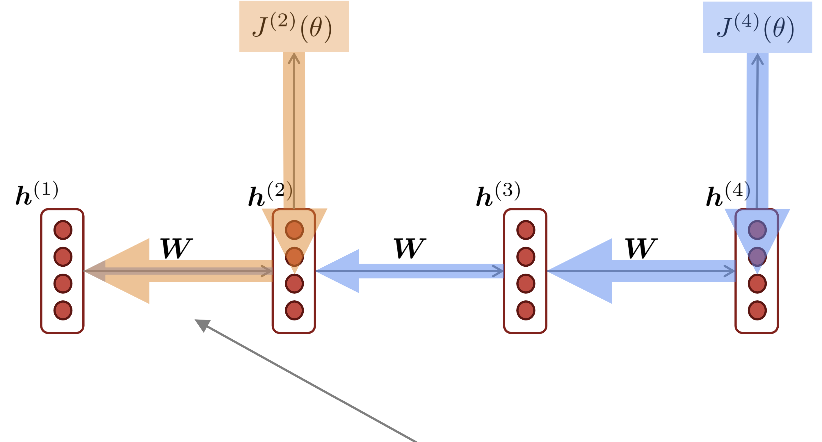
Reference. Stanford CS224n, 2021: Gradient signal from far away is lost because it’s much smaller than gradient signal from close-by. So, model weights are updated only with respect to near effects, not long-term effects.
- Effect of vanishing gradient on RNN-LM
- LM task: When she tried to print her tickets, she found that the printer was out of toner. She went to the stationery store to buy more toner. It was very overpriced. After installing the toner into the printer, she finally printed her ____
- To learn from this training example, the RNN-LM needs to model the dependency between “tickets” on the 7th step and the target word “tickets” at the end.
- But if gradient is small, the model can’t learn this dependency
- So, the model is unable to predict similar long-distance dependencies at test time
- Reference
2.2 Exploding gradients
If the gradient becomes too big, then the SGD update step becomes too big:
\[\theta^{new} = \theta^{old}-\alpha\nabla_{\theta}J(\theta), \alpha\text{: learning rate}, \nabla_{\theta}J(\theta)\text{: gradient}\]This can cause bad updates: we take too large a step and reach a weird and bad parameter configuration (with large loss). In the worst case, this will result in Inf or NaN in your network(then you have to restart training from an earlier checkpoint).
2.3 Gradient clipping: solution for exploding gradient
Gradient clipping: if the norm of the gradient is greater than some threshold, scale it down before applying SGD update
Algorithm 1 Pseudo-code for norm clipping
\[\begin{aligned} &\hat g \leftarrow \dfrac{\partial \varepsilon}{\partial \theta}\\ &\text{if} \lvert\lvert\hat g\lvert\lvert \geq \text{threshold}, \text{ then}\\ &\qquad\hat g \leftarrow \dfrac{threshold}{\lvert\lvert\hat g\lvert\lvert}\hat g \\ &\text{end if} \end{aligned}\]Intuition: take a step in the same direction, but a smaller step. In practice, remembering to clip gradients is important, but exploding gradients are an easy problem to solve
$\checkmark$ How to fix the vanishing gradient problem?
The main problem is that it’s too difficult for the RNN to learn to preserve information over many time steps. In a vanilla RNN, the hidden state is constantly being rewritten
\[h^{(t)} = \sigma(W_h h^{(t-1)} +W_x x^{(t)}+b)\]How about a RNN with separate memory?
3. GRU Gated Recurrent Units
So far, we have discussed methods that transition from hidden state $h_{t−1}$ to $h_t$ using an affine transformation and a point-wise nonlinearity. Here, we discuss the use of a gated activation function thereby modifying the RNN architecture. What motivates this? Well, although RNNs can theoretically capture long-term dependencies, they are very hard to actually train to do this. Gated recurrent units are designed in a manner to have more persistent memory thereby making it easier for RNNs to capture long-term dependencies.
Let us see mathematically how a GRU uses $h_{t-1}$ and $x_t$ to generate the next hidden state $h_t$. We will then dive into the intuition of this architecture.
\[\begin{aligned} z_t &= \sigma(W^{(z)}x_t + U^{(z)}h_{t-1}) &\text{Update gate}\\ r_t &= \sigma(W^{(r)}x_t + U^{(r)}h_{t-1}) &\text{Reset gate}\\ \hat{h}_t &= tanh(r_t \odot Uh_{t-1}+Wx_t) &\text{New memory}\\ h_t &= (1-z_t)\odot \hat{h}_t + z_t \odot h_{t-1} &\text{Hidden state}\\ \end{aligned}\]The above equations can be thought of a GRU’s four fundamental operational stages and they have intuitive interpretations that make this model much more intellectually satisfying (see Figure):
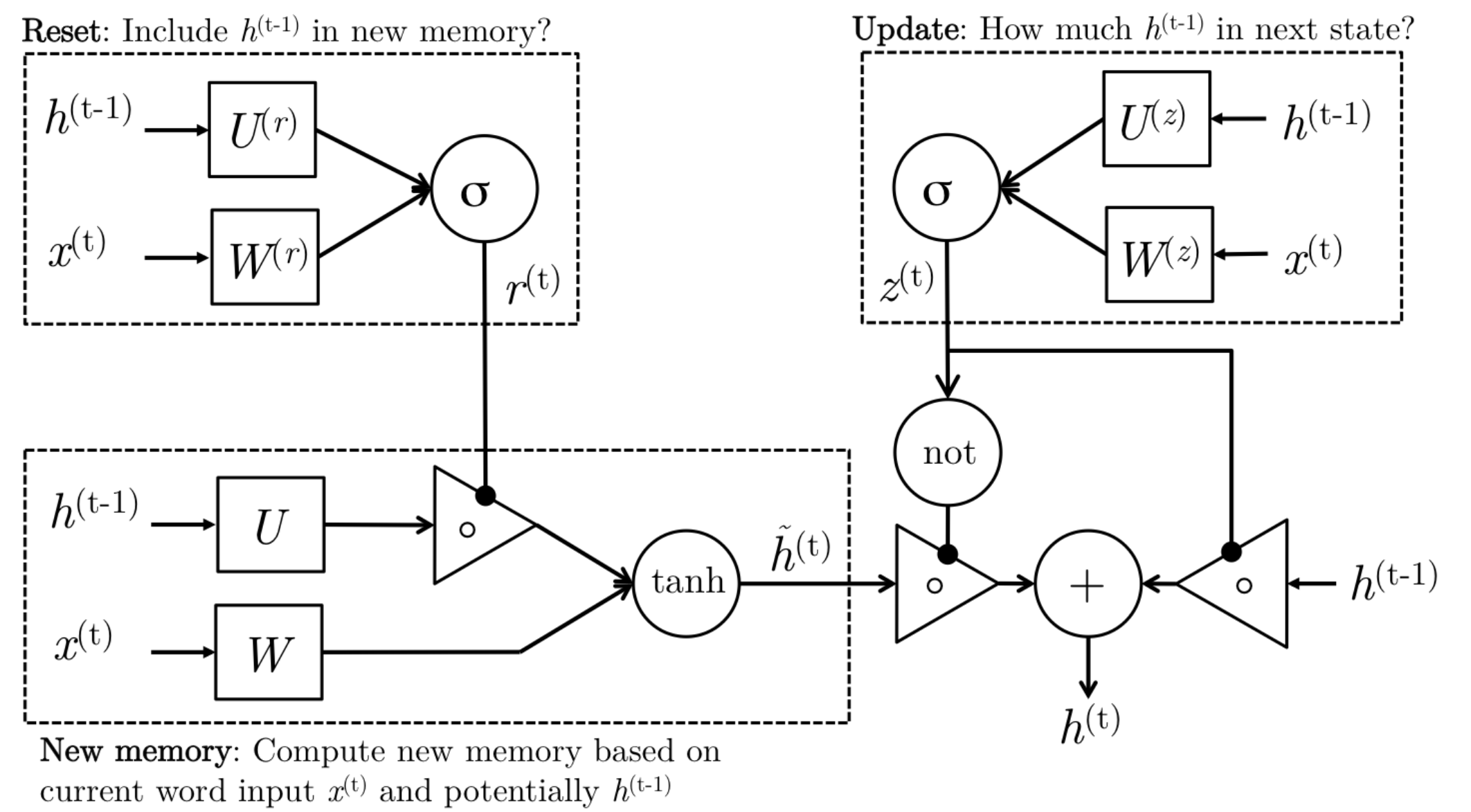
Reference. Stanford CS224n, Figure: The detailed internals of a GRU
1. New memory generation: A new memory $\tilde h_t$ is the consolidation of a new input word xt with the past hidden state $h_{t−1}$. Anthropomorphically, this stage is the one who knows the recipe of combining a newly observed word with the past hidden state $h_{t−1}$ to summarize this new word in light of the contextual past as the vector $\tilde h_t$.
2. Reset Gate: The reset signal $r_t$ is responsible for determining how important ht−1 is to the summarization $\tilde h_t$. The reset gate has the ability to completely diminish past hidden state if it finds that $h_{t−1}$ is irrelevant to the computation of the new memory.
3. Update Gate: The update signal $z_t$ is responsible for determining how much of $h_{t−1}$ should be carried forward to the next state. For instance, if $z_t ≈ 1$, then $h_{t−1}$ is almost entirely copied out to $h_t$. Conversely, if $z_t ≈ 0$, then mostly the new memory $\tilde h_t$ is forwarded to the next hidden state.
4. Hidden state: The hidden state $h_t$ is finally generated using the past hidden input $h_{t−1}$ and the new memory generated $\tilde h_t$ with the advice of the update gate.
4. LSTM Long Short Term Memories
A type of RNN proposed by Hochreiter and Schmidhuber in 1997 as a solution to the vanishing gradients problem. Everyone cites that paper but really a crucial part of the modern LSTM is from Gersetal.(2000)💜
On step t, there is a hidden state $h^{(t)}$and a cell state $c^{(t)}$
- Both are vectors length n
- The cell stores
long-term information - The LSTM can
read, erase, and writeinformation from the cell- The cell becomes conceptually rather like RAM in a computer
The selection of which information is erased/written/read is controlled by three corresponding gates
- The gates are also vectors length n
- On each time step, each element of the gates can be open(1), closed(0), or some where in-between
- The gates are dynamic: their value is computed based on the current context
We have a sequence of inputs $x^{(t)}$, and we will compute a sequence of hidden states $h^{(t)}$ and cell states $c^{(t)}$. On timestep t:
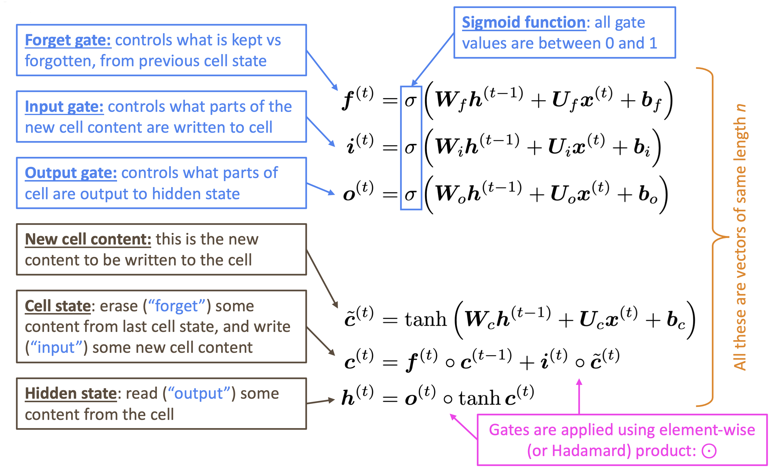
Reference. Stanford CS224n
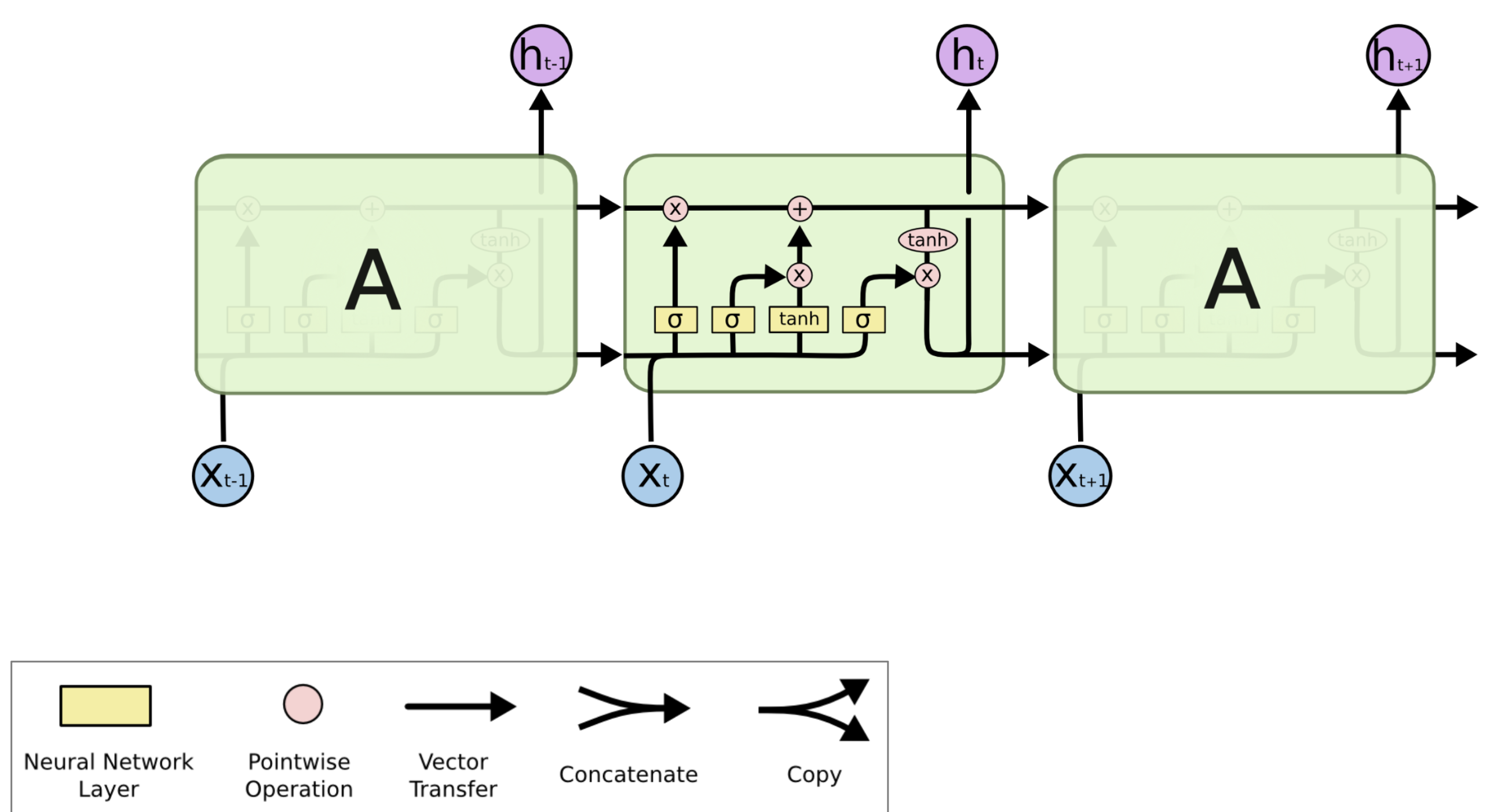
Reference. Stanford CS224n
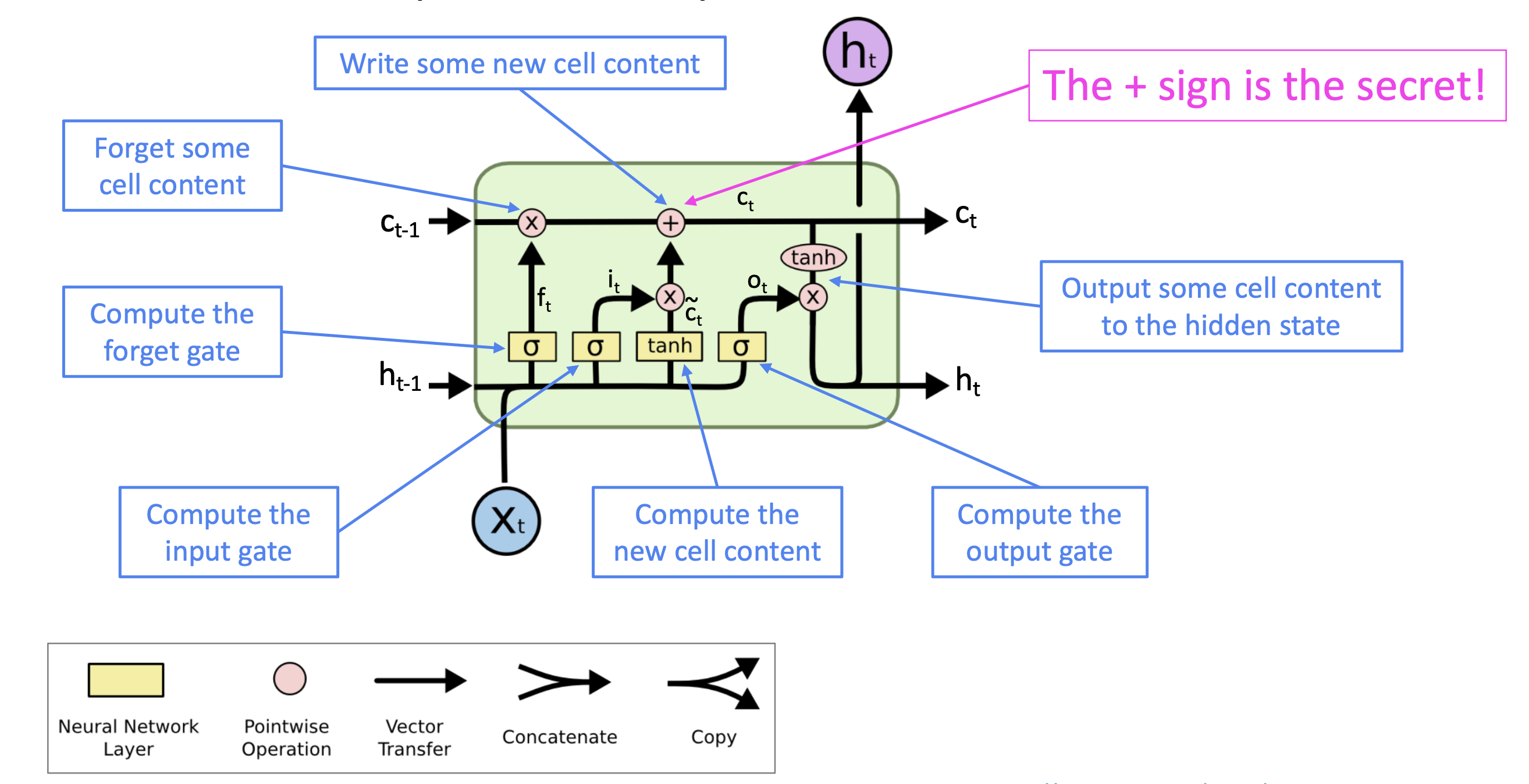
Reference. Stanford CS224n
4.1 LSTM Block Diagram and Explanation
Long-Short-Term-Memories are another type of complex activation unit that differ a little from GRUs. The motivation for using these is similar to those for GRUs however the architecture of such units does differ. Let us first take a look at the mathematical formulation of LSTM units before diving into the intuition behind this design:
\[\begin{aligned} i_t &= \sigma (W^{(i)}x_t + U^{(i)}h_{t-1}) &\text{(Input gate)} \\ f_t &= \sigma (W^{(f)}x_t + U^{(f)}h_{t-1}) &\text{(Forget gate)} \\ o_t &= \sigma (W^{(o)}x_t + U^{(o)}h_{t-1}) &\text{(Output/Exposure gate)} \\ \hat{c}_t &= tanh (W^{(c)}x_t + U^{(c)}h_{t-1}) &\text{(New memory cell)} \\ c_t &= f_t \odot c_{t-1}) + i_t \odot \hat{c_t} &\text{(Final memory cell)} \\ h_t &= o_t \odot tanh(c_t) \\ \end{aligned}\]
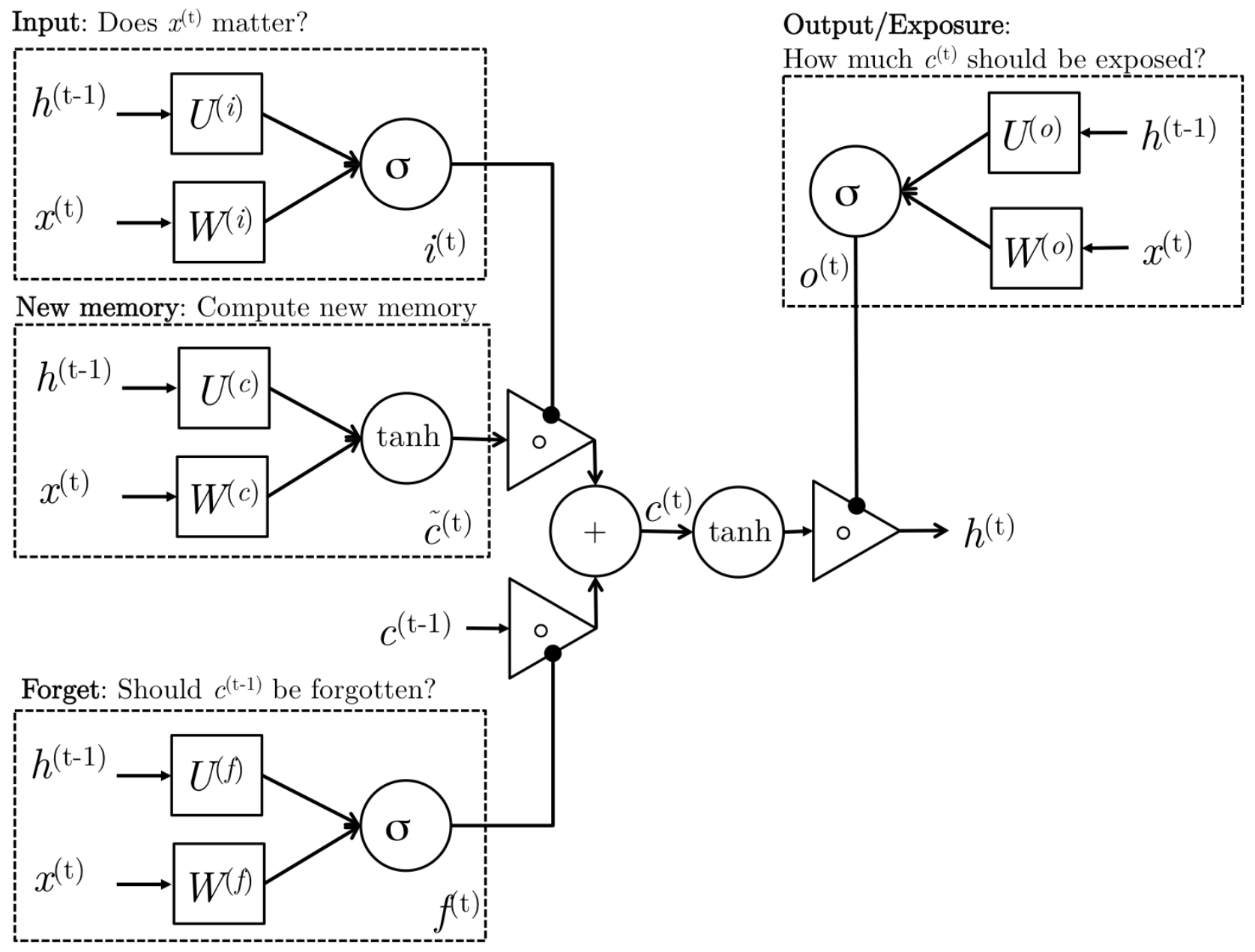
Reference. Stanford CS224n, The detailed internals of a LSTM
We can gain intuition of the structure of an LSTM by thinking of its architecture as the following stages:
-
New memory generation: This stage is analogous to the new memory generation stage we saw in GRUs. We essentially use the input word $x_t$ and the past hidden state $h_{t−1}$ to generate a new memory $\tilde c_t$ **which includes aspects of the new word $x(t)$.
-
Input Gate: We see that the new memory generation stage doesn’t check if the new word is even important before generating the new memory – this is exactly the input gate’s function. The input gate uses the input word and the past hidden state to determine whether or not the input is worth preserving and thus is used to gate the new memory. It thus produces $i_t$ **as an indicator of this information.
-
Forget Gate: This gate is similar to the input gate except that it does not make a determination of usefulness of the input word – instead it makes an assessment on whether the past memory cell is useful for the computation of the current memory cell. Thus, the forget gate looks at the input word and the past hidden state and produces $f_t$.
-
Final memory generation: This stage first takes the advice of the forget gate $f_t$ *and accordingly forgets the past memory $c_{t−1}$. Sim- ilarly, it takes the advice of the input gate it* and accordingly gates the new memory $\tilde c_t$. It then sums these two results to produce the final memory $c_t$.
-
Output/Exposure Gate: This is a gate that does not explicitly exist in GRUs. It’s purpose is to separate the final memory from the hidden state. The final memory $c_t$ contains a lot of information that is not necessarily required to be saved in the hidden state. Hidden states are used in every single gate of an LSTM and thus, this gate makes the assessment regarding what parts of the memory $c_t$ needs to be exposed/present in the hidden state $h_t$. The signal it produces to indicate this is $o_t$ and this is used to gate the point-wise tanh of the memory.
-
How does LSTM solve vanishing gradients?
The LSTM architecture makes it easier for the RNN to preserve information over many timesteps
-
e.g., if the forget gate is set to 1 for a cell dimension and the input gate set to 0, then the information of that cell is preserved indefinitely.
-
In contrast, it’s harder for a vanilla RNN to learn a recurrent weight matrix $W_h$ that preserves info in the hidden state
-
In practice, you get about 100 timesteps rather than about 7
LSTM doesn’t guarantee that there is no vanishing/exploding gradient, but it does provide an easier way for the model to learn long-distance dependencies.
$\checkmark$ Reference
- “Long short-term memory”, Hochreiter and Schmidhuber, 1997.
- “Learning to Forget: Continual Prediction with LSTM”, Gers, Schmidhuber, and Cummins, 2000.
- Diagram, http://colah.github.io/posts/2015-08-Understanding-LSTMs/
$\checkmark$ LSTMs: Success in real word
In 2013–2015, LSTMs started achieving state-of-the-art results
- Successful tasks include handwriting recognition, speech recognition, machine translation, parsing, and image captioning, as well as language models
- LSTMs became the dominant approach for most NLP tasks
Now (2021), other approaches (e.g., Transformers) have become dominant for many tasks
- For example, in WMT (a Machine Translation conference + competition):
- In WMT 2016, the summary report contains “RNN” 44 times
- In WMT 2019: “RNN” 7 times, ”Transformer” 105 times
- Source: “Findings of the 2019 Conference on Machine Translation (WMT19)”, Barrault et al. 2019
5. Is vanishing/exploding gradient just RNN problem?
No! It can be a problem for all neural architectures (including feed-forward and convolutional), especially very deep ones.
- Due to chain rule/ choice of nonlinearity function, gradient can become vanishingly small as it backpropagates
- Thus, lower layers are learned very slowly(hard to train)
Solution: lots of new deep feedforward/ convolutional architectures that add more direct connections (thus allowing the gradient to flow)
5.1 Example for solution
$\checkmark$ “ResNet”
- Residual connections aka “ResNet”
- Also known as skip-connections
- The identity connection preserves information by default
- This makes deep networks much easier to train
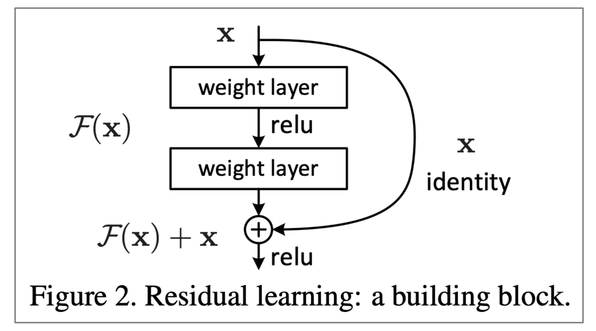
"Deep Residual Learning for Image Recognition", He et al, 2015.
$\checkmark$ “DenseNet”
- Dense connections aka “DenseNet”
- Directly connect each layer to all future layers!
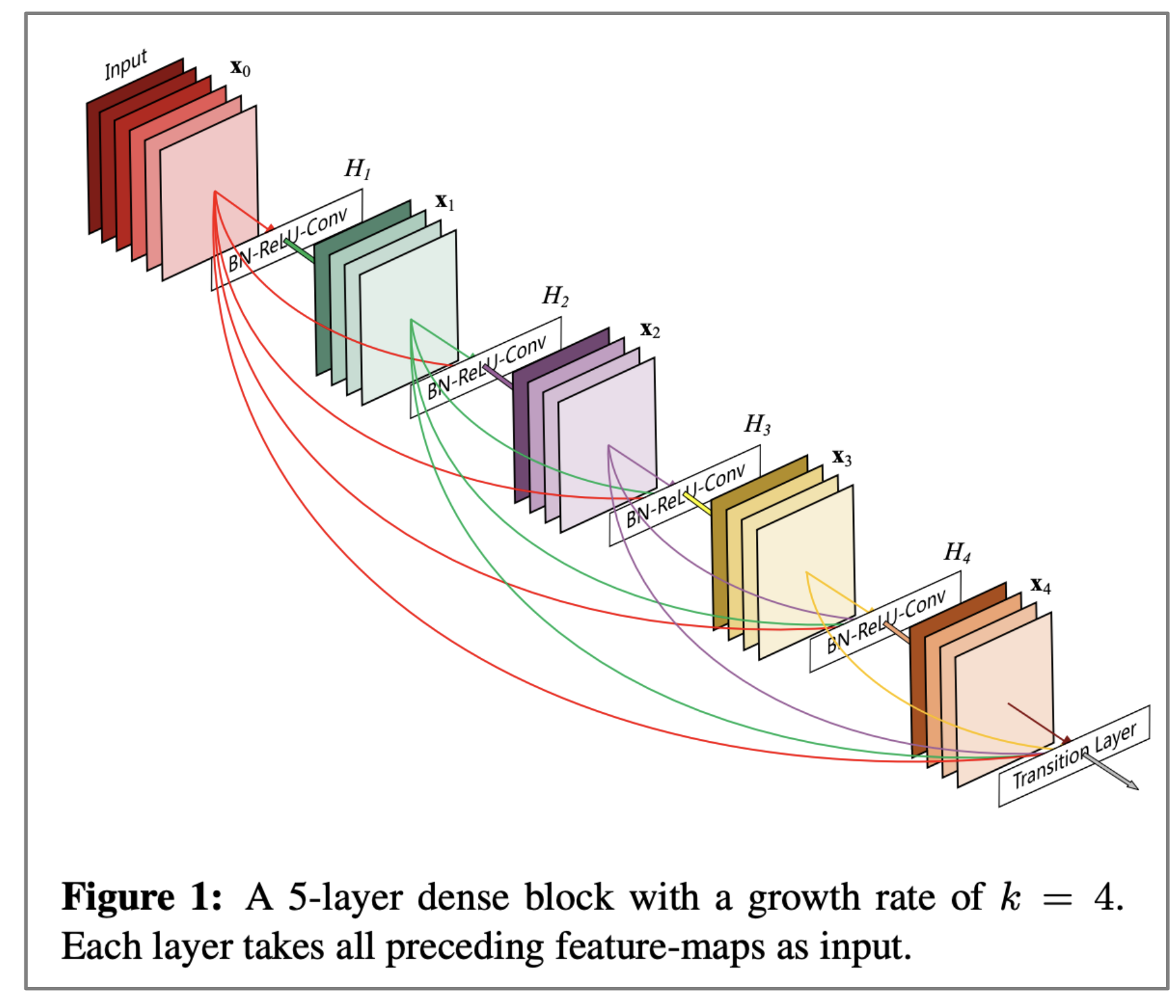
”Densely Connected Convolutional Networks", Huang et al, 2017.
$\checkmark$ “HighwayNet”
- Highway connections aka “HighwayNet”
- Similar to residual connections, but the identity connection vs the transformation layer is controlled by a dynamic gate
- Inspired by LSTMs, but applied to deep feedforward/convolutional networks
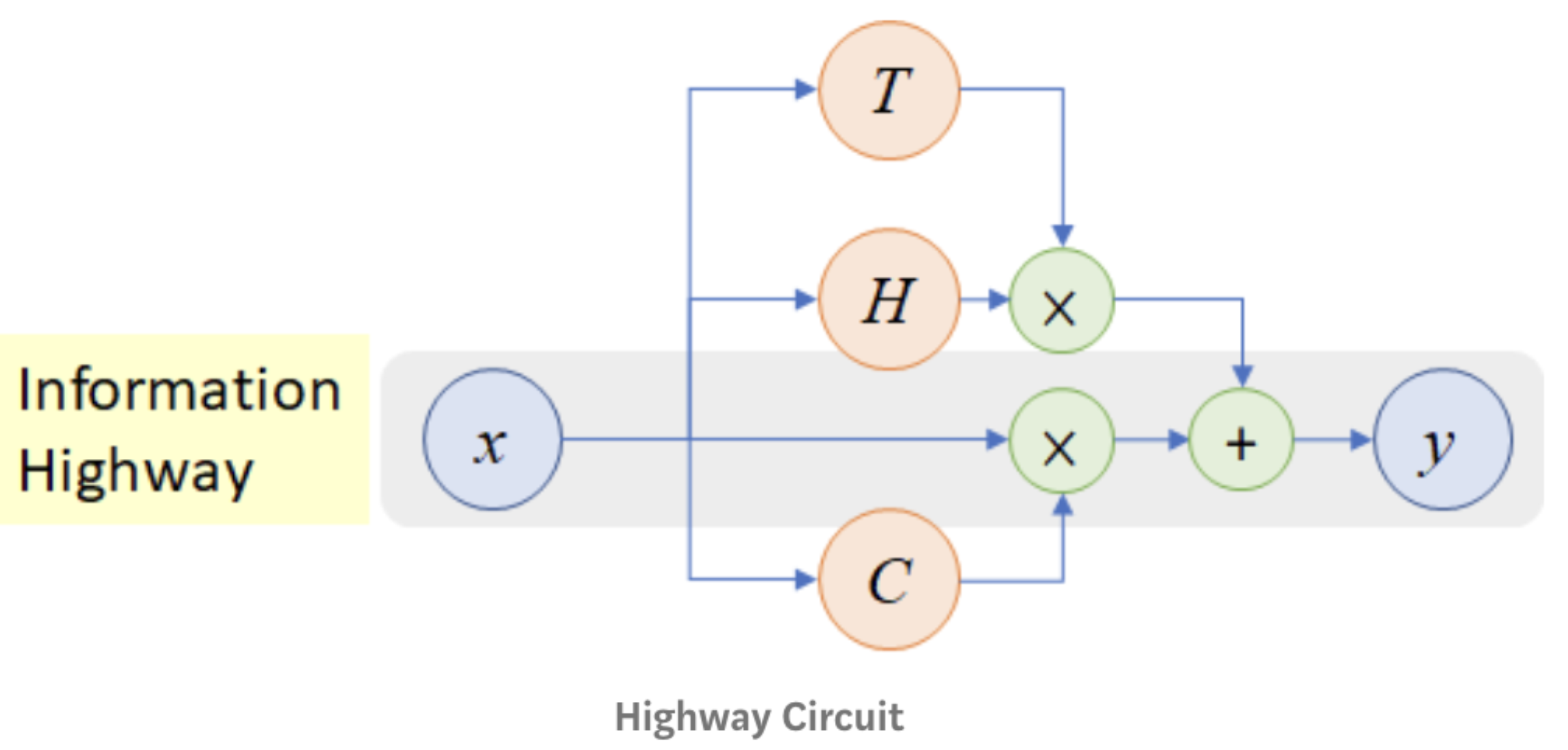
”Highway Networks", Srivastava et al, 2015.
Conclusion: Though vanishing/exploding gradients are a general problem, RNNs are particularly unstable due to the repeated multiplication by the same weight matrix [Bengio et al, 1994]
Reference
- “Deep Residual Learning for Image Recognition”, He et al, 2015.]
- ”Densely Connected Convolutional Networks”, Huang et al, 2017.
- ”Highway Networks”, Srivastava et al, 2015.]
- ”Learning Long-Term Dependencies with Gradient Descent is Difficult”, Bengio et al. 1994
6. Bidirectional RNN
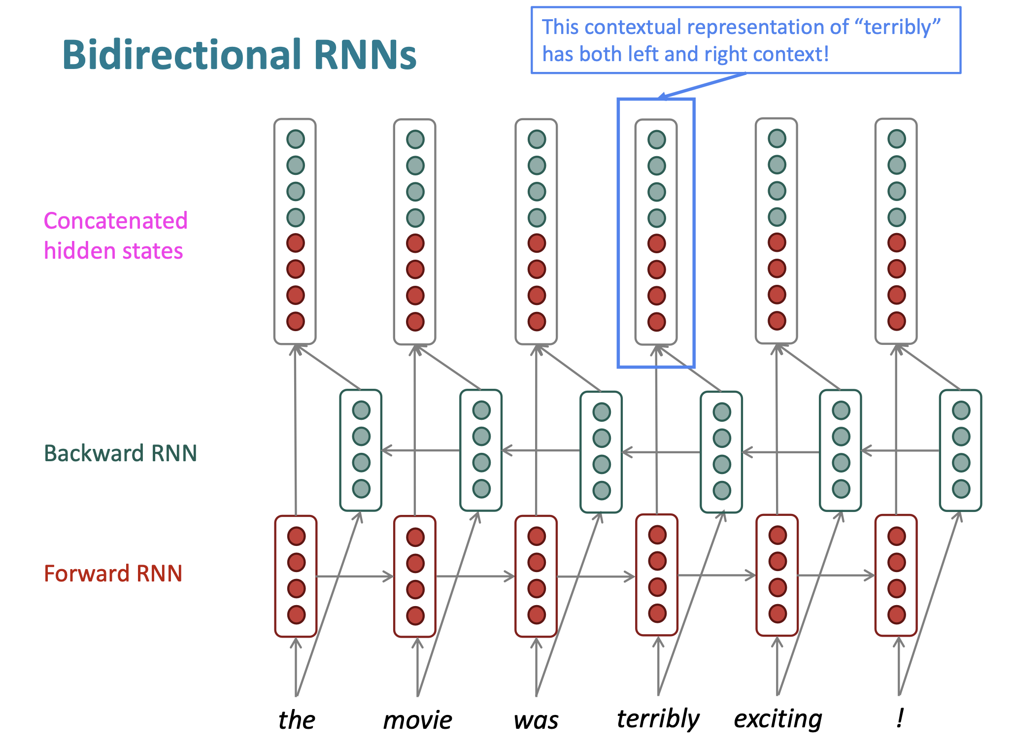
- Motivation: The contextual representation such as “terribly” has both left and right context
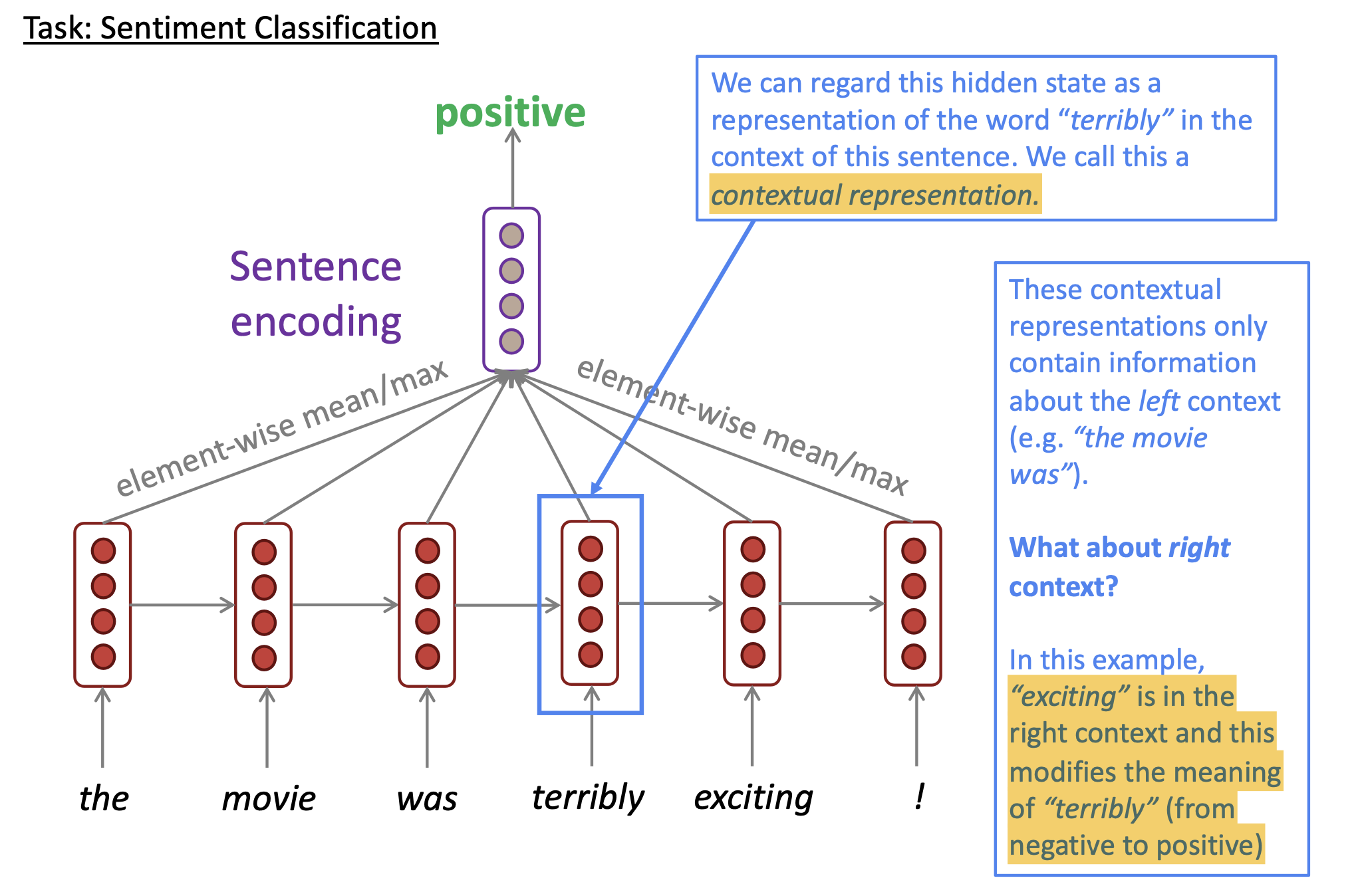
Reference. Stanford CS224n
Reference. Stanford CS224n
On timestep t:
Forward RNN: $\overrightarrow{h}^{(t)}=RNN_{FW}(\overrightarrow{h}^{(t-1)}, x^{(t)}) = f(\overrightarrow Wx_t +\overrightarrow V \overrightarrow h_{t-1} + \overrightarrow b)$
Backward RNN: $\overleftarrow{h}^{(t)}=RNN_{FW}(\overleftarrow{h}^{(t+1)}, x^{(t)}) = f(\overleftarrow Wx_t +\overleftarrow V \overleftarrow h_{t-1} + \overleftarrow b)$
Concatenated hidden states $h^{(t)} = [\overrightarrow{h}^{(t)};\overleftarrow{h}^{(t)}]$
$\hat y = g(Uh_t+c)=g(U[\overrightarrow h_t; \overleftarrow h_t]+c)$
$RNN_{FW}$: This is a general notation to mean “compute one forward step of the RNN” – it could be a vanilla, LSTM or GRU computation.
$h^{(t)}$: We regard this as “the hidden state” of a bidirectional RNN. This is what we pass on to the next parts of the network.
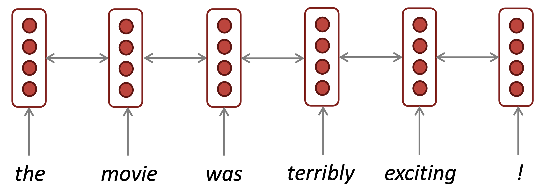
Reference. Stanford CS224n
The two-way arrows indicate bidirectionality and the depicted hidden states are assumed to be the concatenated forwards+backwards states.
Note: bidirectional RNNs are only applicable if you have access to the entire input sequence. They are not applicable to Language Modeling, because in LM you only have left context available. If you do have entire input sequence (e.g., any kind of encoding), bidirectionality is powerful (you should use it by default). For example, BERT (Bidirectional Encoder Representations from Transformers) is a powerful pretrained contextual representation system built on bidirectionality.
7. Multi-layer RNN
We can also make them “deep” in another dimension by applying multiple RNNs – this is a multi-layer RNN. Multi-layer RNNs are also called stacked RNNs. High-performing RNNs are often multi-layer (but aren’t as deep as convolutional or feed-forward networks)
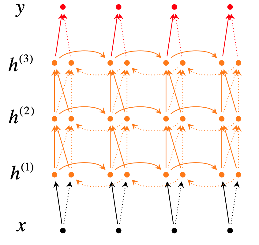
Reference. Stanford CS224n, Figure: A deep bi-directional RNN with three RNN layers.
\[\begin{aligned} \overrightarrow h_t^{(i)} &= f(\overrightarrow W^{(i)}h_t^{(i-1)}+\overrightarrow V^{(i)}\overrightarrow h_{t-1}^{(i)}+\overrightarrow b^{(i)}) \\ \overleftarrow h_t^{(i)} &= f(\overleftarrow W^{(i)}h_t^{(i-1)}+\overleftarrow V^{(i)}\overleftarrow h_{t-1}^{(i)}+\overleftarrow b^{(i)}) \\ \hat y &= g(Uh_t+c)=g(U[\overrightarrow h_t^{(L)}; \overleftarrow h_t^{(L)}]+c) \end{aligned}\]For example: In 2017 paper, Britz et al find that for Neural Machine Translation, 2 to 4 layers is best for the encoder RNN, and 4 layers is best for the decoder RNN. Usually,skip-connections/dense connections are needed to train deeper RNNs (e.g.,8 layers). Transformer-based networks (e.g., BERT) are usually deeper, like 12 or 24 layers.
8. Summary
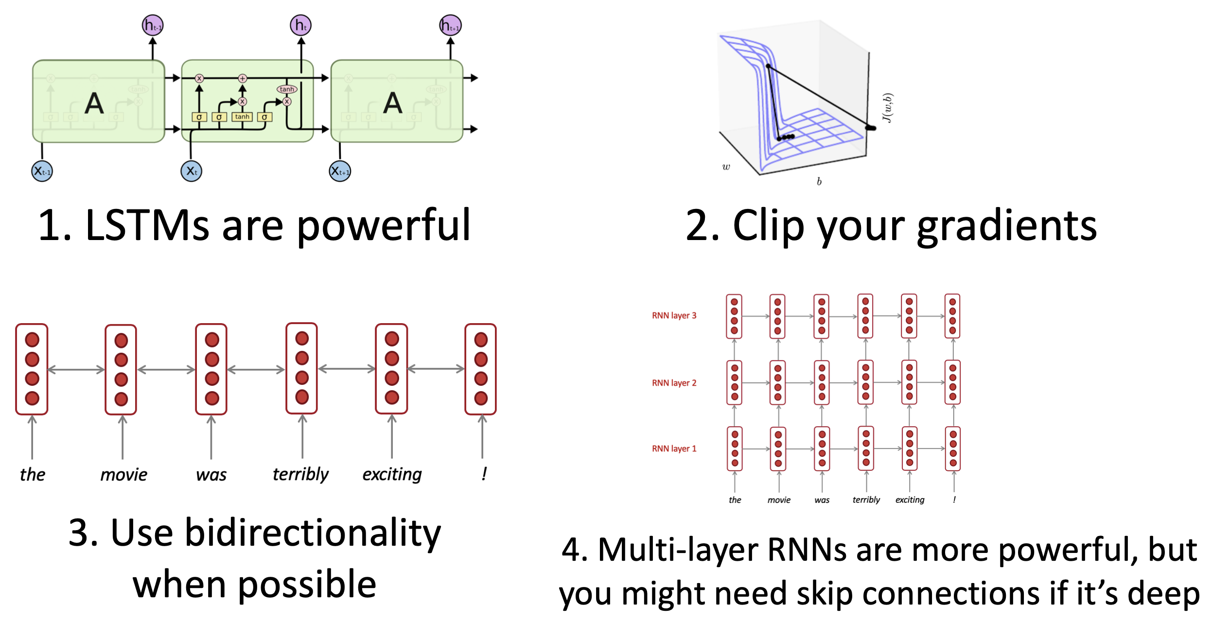
Reference. Stanford CS224n, http://web.stanford.edu/class/cs224n/
(Paper) Initialization
- Paper. Delving deep into rectifiers surpassing human level performance on imagenet classification
$\checkmark$ Sigmoid → Xavier Initialization
-
Why’s Xavier initialization important?
If the weights in a network start too small, then the signal shrinks as it passes through each layer until it’s too tiny to be useful.
If the weights in a network start too large, then the signal grows as it passes through each layer until it’s too massive to be useful.
-
What’s Xavier initialization?
In Caffe, it’s initializing the weights in your network by drawing them from a distribution with zero mean and a specific variance,
\[Var(W)=\dfrac{1}{n_{in}}\]where W is the initialization distribution for the neuron in question, and ninnin is the number of neurons feeding into it. The distribution used is typically Gaussian or uniform.
It’s worth mentioning that Glorot & Bengio’s paper originally recommended using
\[Var(W)=\dfrac{2}{n_{in}+n_{out}}\]where noutnout is the number of neurons the result is fed to. We’ll come to why Caffe’s scheme might be different in a bit.
-
Where did those formulas come from? Refer to Ref1. Blog**
$\checkmark$ Reference
- https://andyljones.tumblr.com/post/110998971763/an-explanation-of-xavier-initialization
- Understanding the difficulty of training deep feedforward neural networks- Glorot, X. & Bengio, Y. (2010)
$\checkmark$ ReLU → He initialization