Optimization for tiny devices in C++ 2/2

지난 번 글부터 Tiny device에 적용할 수 있는 ML 최적화 기법에 대해 정리하고 있다. 이번 글에서는 Image to Column(Im2col) convolution, In-place depth-wise convolution, NHWC for point-wise convolution, and NCHW for depth-wise convolution, Winograd convolution를 다룰 예정이고, 저번 시간에 이어 그에 맞는 예제를 직접 보드에서 돌려보면서 어떻게 최적화가 되는지 알아보자.

3.5 Image to Column(Im2col) convolution

Im2col는 데이터를 행렬형태로 재배치하여 Generalized Matrix Multiplication(GEMM)을 이용해서 convolution을 연산하는 방식이다. 아래 간단하게 예제를 들어보자.

크기가 4인 input image f와 크기가 3인 filter g이 있다고 하면 다음과 같이 표현할 수 있다.

이걸 Im2col 기법을 사용하게 되면 f를 2x3 행렬에 convolution 연산을 하기위해 데이터를 담는 것이다.

이렇게 데이터를 재배치하면 GEMM과 같이 행렬연산자체의 최적화를 통해 성능을 높일 수 있는 것이다. 그럼 GEMM은 어떤 방식인데? 이것에 대해서는 내용이 길기에 이 글을 참고하자. 하지만 GEMM을 사용하면 행렬로 펼친 데이터 만큼의 메모리 공간이 추가로 필요하다. 그래서 이 문제를 해결하기 위한 방법으로 CuBLAS (GPU), Intel MKL(CPU), 와 같은 BLAS(Basic Linear Algebra Subprograms) 라이브러리와 Nvidia의 Tensor core가 있다.

Reference. MIT-TinyML-lecture17-TinyEngine in https://efficientml.ai

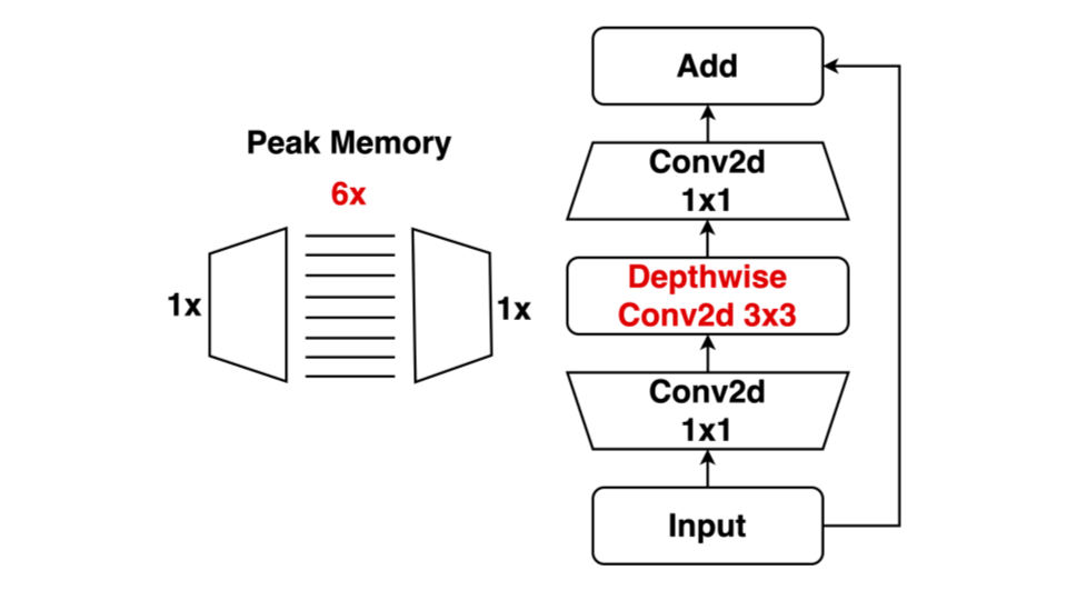
3.6 In-place depth-wise convolution: Reduce peak memory

In-place depth-wise convolution은 아래와 같은 Depth-wise convolution 연산한 결과를 입력 데이터에 덮어써서 Peak memory를 줄이는 방식이다. 두 번째 그림을 보면 이해하기 더 쉽다.

Reference. MIT-TinyML-lecture17-TinyEngine in https://efficientml.ai

Reference. MIT-TinyML-lecture17-TinyEngine in https://efficientml.ai

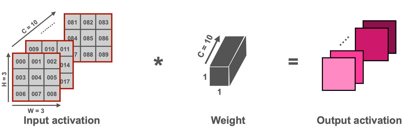
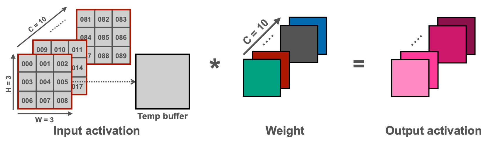
3.7 NHWC for point-wise convolution, and NCHW for depth-wise convolution

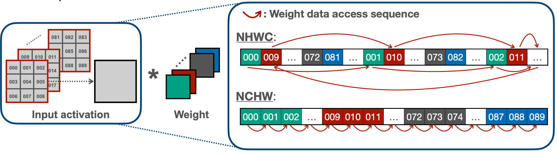
NHWC와 NCHW는 각각 point-wise convolution과 depth-wise convolution 연산에 맞게 포인터를 이동하여 데이터를 읽기 순차적으로 읽기 위해 데이터 배열을 바꾸는 방법이다. 여기서 N은 배치사이즈, C는 채널, 그리고 H와 W는 이미지의 높이(Height)와 너비(Width)가 되겠다. 이 방법 역시 캐시를 이용하는 것이 핵심인데, NCHW의 경우 point-wise convolution연산을 위해 NHWC로 바꾸면 아래 두 번쨰 그림과 같이 데이터를 읽을 수 있다.

Reference. MIT-TinyML-lecture17-TinyEngine in https://efficientml.ai

Reference. MIT-TinyML-lecture17-TinyEngine in https://efficientml.ai

그리고 NHWC의 경우 depth-wise convolution연산을 위해 NCHW로 바꾸면 아래 두 번째 그림과 같이 데이터를 메모리에서 순차적으로 읽을 수 있다.

Reference. MIT-TinyML-lecture17-TinyEngine in https://efficientml.ai

Reference. MIT-TinyML-lecture17-TinyEngine in https://efficientml.ai

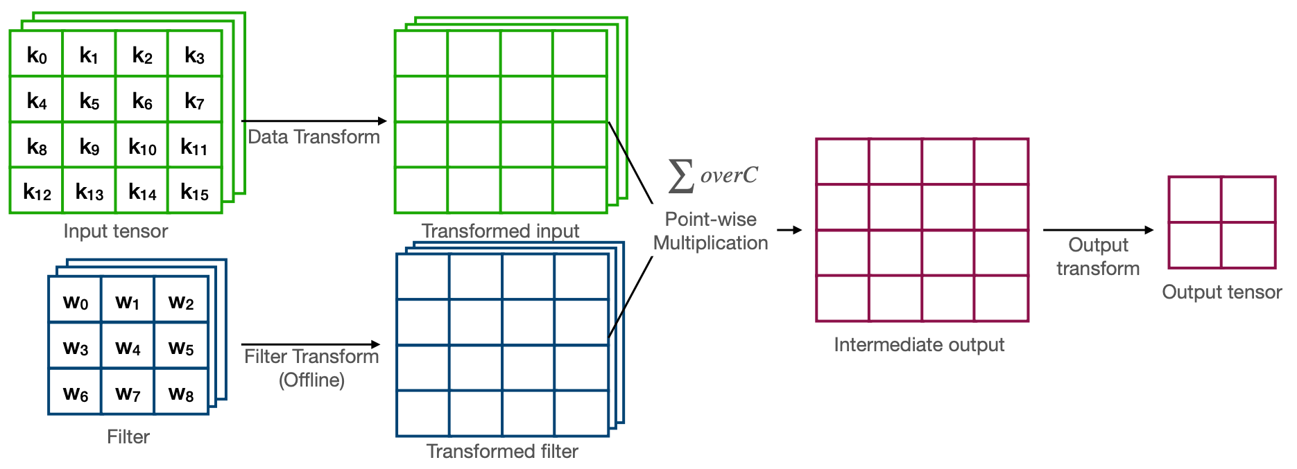
3.8 Winograd convolution

기존에 아래와 같은 Convolution으로 연산하게되면 4개의 output을 위해서 9xCx4 MACs 연산이 필요하다.

Reference. MIT-TinyML-lecture17-TinyEngine in https://efficientml.ai

Reference. MIT-TinyML-lecture17-TinyEngine in https://efficientml.ai

Winograd convolution은 이를 16xC MACs 연산수만큼 줄여 2.25x 배 더 적은 연산 수로 Convolution을 할 수 있다.

음, 간단하게 Im2col에서 사용했던 예제를 다시 가져와보자. 크기가 4인 input image f와 크기가 3인 filter g이 있다고 하고 Im2col기법을 사용하면 다음과 같이 표현할 수 있다.

여기서 결과를 계산해보면,

이를 일반화 하면,

그럼 m1, m2, m3, m4는 다음과 같이 표현할 수 있다.

이걸 그림으로 표현한 것이 아래 그림!

Reference. MIT-TinyML-lecture17-TinyEngine in https://efficientml.ai

여기서 g0, g1, g2의 경우 filter이므로 g0+g1+g2와 같은 경우를 미리 계산한다고 하면 convolution에 사용하는 연산은 4xADD 연산과 4xMUL 연산이 된다. 이는 6xMUL 연산이 필요한 기존의 방식보다 1.5x 더 적은 연산 수로 Convolution을 할 수 있다는 것이다.

위의 예제처럼 만약 convolution을 input f(4,4)와 filter g(3,3)을 한다고 하면 기존에 연산은 229=36 MUL인 반면 Winograd convolution은 4*4=16 MUL로 2.25x 더 적은 연산 수로 Convolution을 할 수 있는 것이다.

3.9 Example of Im2col, In-place depth-wise convolution, and NCHW for depth-wise convolution

첫 번째로 작업은 Im2col을 위해 데이터 배열을 바꾸는 것이다. “테두리에 padding을 하고 사각형을 source(src)로 부터 만든다.” 고 생각하면서 코드를 봐보자.

tinyengine_status depthwise_kernel3x3_stride1_inplace_CHW(q7_t *input, const uint16_t input_x, const uint16_t input_y,
				const uint16_t input_ch, const q7_t *kernel, const int32_t *bias, const int32_t *biasR,
				const int32_t *output_shift, const int32_t *output_mult,
				const int32_t output_offset, const int32_t input_offset,
				const int32_t output_activation_min,
				const int32_t output_activation_max, q7_t *output,
				const uint16_t output_x, const uint16_t output_y,
				const uint16_t output_ch, q15_t *runtime_buf, q7_t pad_value) {
    uint16_t c,i,j;
	q7_t *cols_8b_start = (q7_t *)runtime_buf;
	q7_t* cols_8b = (q7_t* )cols_8b_start;

	//Set padding value
	q7_t PAD8 = pad_value;
	/* setup the padding regions for Im2col buffers */
	//top region: 8bit x (input_x + pad_w * 2) x pad_h: unroll by pad value
	for(i = 0; i < input_x + 2; i++){
		*cols_8b++ = PAD8;
	}

	//middle regions: left and right regions
	for(i = 0; i < input_y; i++){
		*cols_8b++ = PAD8;  //left
		cols_8b += input_x; //skip middle
		*cols_8b++ = PAD8;  //right
	}

	//bottom region: 8bit x (input_x + pad_w * 2) x pad_h: unroll by pad value
	for(i = 0; i < input_x + 2; i++){
		*cols_8b++ = PAD8;
	}

	const q7_t *src;
	const q7_t *ksrc = kernel;

	for (c = 0; c < input_ch; c++){
        cols_8b = (q7_t*)(cols_8b_start + 1 * (input_x) + 2); //skip 1 rows
        src = input;
        for(i = 0; i < input_y; i++){
            cols_8b += 1;//skip front
            for(j = 0; j < input_x; j++){
                *cols_8b++ = *src;// + input_offset;
                src += input_ch;
            }
            cols_8b += 1;//skip end
        }

			// ...

이제 이 준비된 데이터 배열을 in-place의 경우 output 포인터에 바로 덮어 쓰면 된다.

#if INPLACE_DEPTHWISE
		q7_t *inplace_out = input;
#else  // if (!INPLACE_DEPTHWISE)
		q7_t *inplace_out = output;
#endif  // end of INPLACE_DEPTHWISE

// ...

#if INPLACE_DEPTHWISE
		input++;
#else  // if (!INPLACE_DEPTHWISE)
		output++;
#endif  // end of INPLACE_DEPTHWISE

// ..

마지막으로 depth-wise convolution을 위해 NCHW로 연산을 하면 된다. 말이 조금 복잡해서 그렇지, 데이터를 순차적으로 읽으면서 연산한다. 그리고 여기에 이전 글에서 다룬 Unrolling을 적용하면 최적화 끝.

tinyengine_status depthwise_kernel3x3_stride1_inplace_CHW(q7_t *input, const uint16_t input_x, const uint16_t input_y,
				const uint16_t input_ch, const q7_t *kernel, const int32_t *bias, const int32_t *biasR,
				const int32_t *output_shift, const int32_t *output_mult,
				const int32_t output_offset, const int32_t input_offset,
				const int32_t output_activation_min,
				const int32_t output_activation_max, q7_t *output,
				const uint16_t output_x, const uint16_t output_y,
				const uint16_t output_ch, q15_t *runtime_buf, q7_t pad_value)
// ...
depthwise_kernel3x3_stride1_inplace_kernel_CHW(output_y, output_x, bias++, biasR++, ksrc, output_mult++, output_shift++, inplace_out, output_offset,output_activation_min, output_activation_max, cols_8b_start, input_x, input_ch);

#if HWC2CHW_WEIGHT
		ksrc += 9;
#else  // if (!HWC2CHW_WEIGHT)
		ksrc++;
#endif  // end of HWC2CHW_WEIGHT
// ...
}

void depthwise_kernel3x3_stride1_inplace_kernel_CHW(
// ...
// channel_offset = input channel
// DIM_KER = KERNEL SIZE (e.g. 3x3 = DIM_KER_X 3 & DIM_KER_Y 3 
#if HWC2CHW_WEIGHT
sum0 += cols_8b[filter_x] * ksrc[filter_y * DIM_KER_X + filter_x];
sum1 += cols_8b[filter_x + 1] * ksrc[filter_y * DIM_KER_X + filter_x];
#else  // if (!HWC2CHW_WEIGHT)
sum0 += cols_8b[filter_x] * ksrc[(filter_y * DIM_KER_X + filter_x) * channel_offset];
sum1 += cols_8b[filter_x + 1] * ksrc[(filter_y * DIM_KER_X + filter_x) * channel_offset];
#endif  // end of HWC2CHW_WEIGHT
// ...

최적화 전후 Frame Per second는 0.447 FPS에서 6.289 ~ 6.329 FPS까지 늘어날 수 있었다. 최적화 기법마다 FPS를 알고싶다면 다시 이전 글로. 그리고, STM32F746G-Discovery보드에서 예제를 돌려본 결과는 다음과 같다. 예제를 돌려보고 싶다면 이 링크를 참고하자.

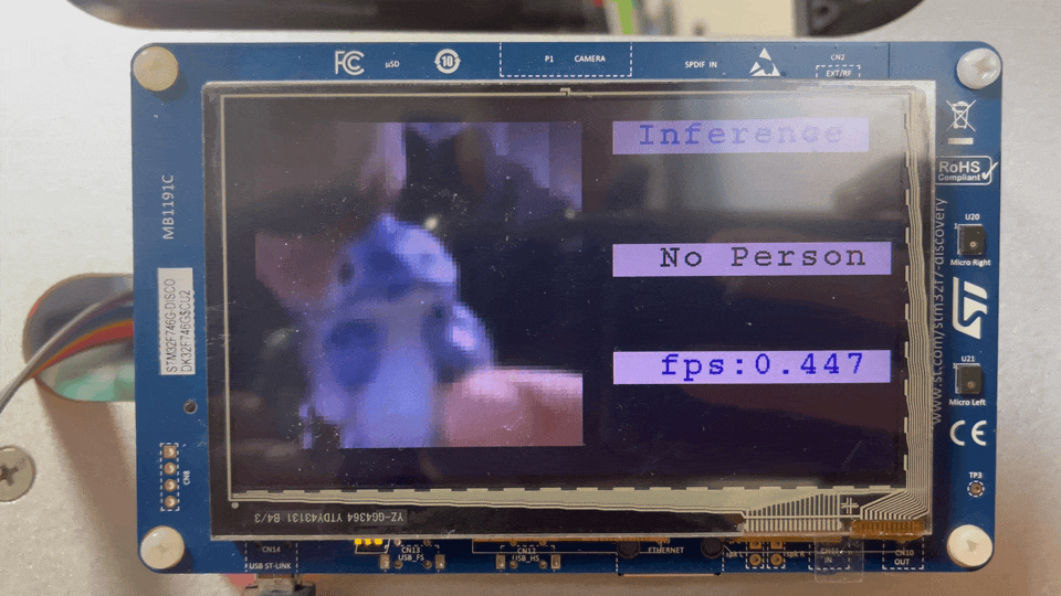
Before applying optimization techniques

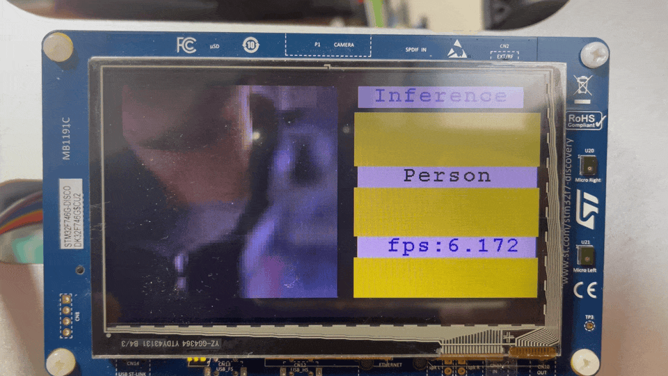
After applying optimization techniques

이번 Tiny Device를 위한 최적화에서는 ML 최적화 기법 중에서 많이 소개되지 않은 Im2col, In-place depth-wise convolution, NHWC for point-wise convolution, and NCHW for depth-wise convolution, Winograd convolution에 대해 알아보았다. 직접 코드를 짜는 경우에 소개해준 방법들이 도움이 되길 바라며, 기법에 초점을 맞추는 것보다 “어떻게 하면 Cache locality를 높일 수 있을까?”에 대해서 하나씩 해결해 나가다 보면 위에 방법들을 다 적용할 수 있지 않을까 싶다.

Reference

• MCUNet: Tiny Deep Learning on IoT Devices [Lin et al., NeurIPS 2020]
• On-Device Training Under 256KB Memory [Lin et al., NeurIPS 2022]
• Im2col: Anatomy of a High-Speed Convolution
• In-place Depth-wise Convolution: MobileNetV2: Inverted Residuals and Linear Bottlenecks [Sandler et al., CVPR 2018]
• Winograd Convolution: “Even Faster CNNs: Exploring the New Class of Winograd Algorithms,” a Presentation from Arm
• Winograd Convolution: Fast Algorithms for Convolutional Neural Networks
• Understanding ‘Winograd Fast Convolution’
• TinyML and Efficient Deep Learning Computing on MIT HAN LAB
• Youtube for TinyML and Efficient Deep Learning Computing on MIT HAN LAB