글에 앞서 본 내용은 MIT 6.006 Introduction to Algorithms, Spring 2020 에서 Binary Tree Part 1, Binary Tree Part 2, 그리고 Binary Heaps을 정리해 둔 것을 우선 말씀드립니다. 본 내용이 영어로 궁금하시면 강의를 꼭 들어보시길 추천드립니다. 그리고 강의 전반으로 각 자료구조에 대해 이야기할 때, 항상 문제 → 자료구조의 정의 → 동작원리(build, insert, delete) → 인터페이스로의 이용(Find) → Sorting(가능하다면) 의 순서로 진행되니 참고 바랍니다.
Reference. MIT 6.006 Introduction to Algorithms, Spring 2020
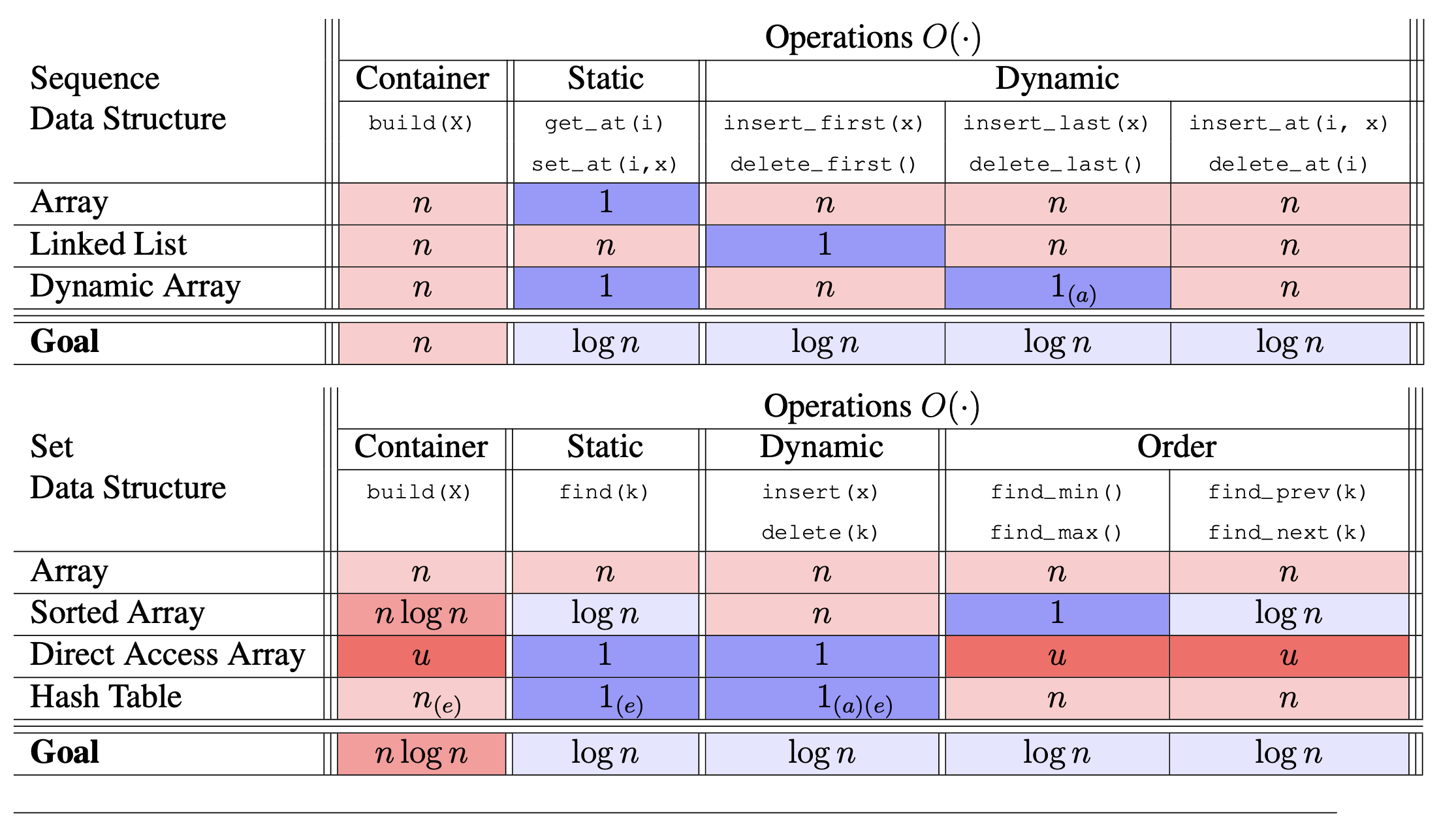
시간 복잡도에서 최고는 역시 $logn$ ! 그럼 모든 operation에서 시간 복잡도 log n을 달성할 수 있는 방법에는 어떤 것이 있을까요? 바로, Binary Tree 입니다. “pointer-based data structure with three pointers per node.” Binary Tree에 대해서 이번 시간에는 이야기해보겠습니다.
1. Word for Binary Tree
Reference. MIT 6.006 Introduction to Algorithms, Spring 2020
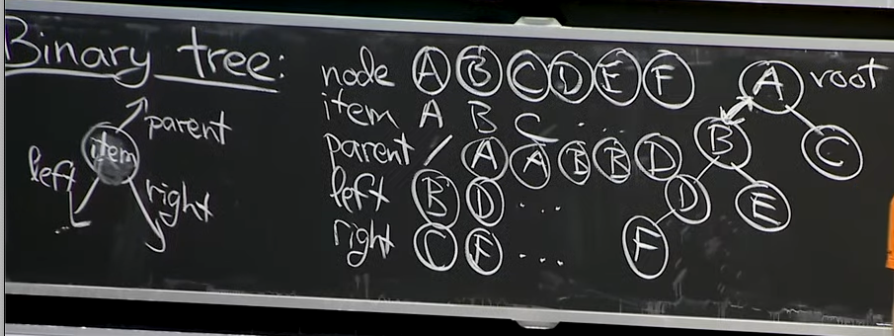
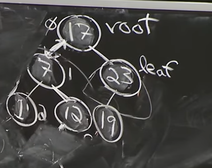
이야기에 앞서 먼저 Binary Tree를 다루면 나오는 용어들입니다.
- Node
- Root
- Parent
- Left/Right
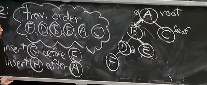
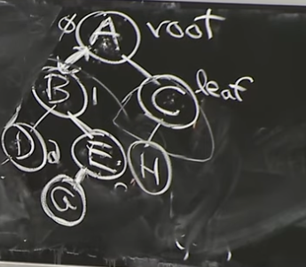
- Leaf: Above picture, Leaf is F, E, C
- Ancestors: Root Node까지 가며 만나는 Node들
- Descendents: Subtree를 그려서 Leaf Node들까지 가며 만나는 Node
- Subtree X : X and its descendents (X is root)
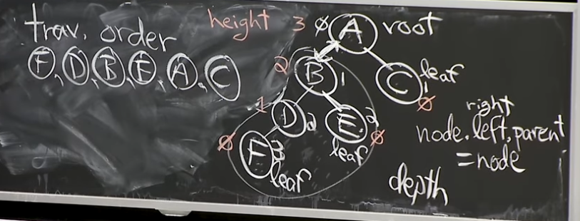
- Depth X: # ancestors = # edges in path form X up to root
- E : Depth 2, B: Depth 1, A: Depth 0 …
- Height X
- #edges in lowest downward path from X
- max depth in subtree X
- F : Height 0, D Height 1, B Height 2 …
- h = height(root) = height(tree)
여기서 h(height)가 자주 나오게 됩니다. “Get O(h) time / op !” 대부분의 Operation에서 O(h)를 가지게 되는 것이 바로 Binary Tree의 가장 큰 특징 이죠. 하지만 아직 log(n)이라고 언급하지 않은 것은, 뒤에 나올 Height Balence가 되지 않았기 때문이죠.
2. Traversal order(In-order)
용어 중 또 하나는 Traversal order, In-order(중위 순회)라고 불리는 방식입니다.
Reference. MIT 6.006 Introduction to Algorithms, Spring 2020
Traversal order는 모든 노드 X에 대해서 노드 X의 왼쪽 노드, 그리고 X, 그리고 오른쪽 X로 표현하는 방식을 말합니다(For every node X, nodes in X.left before X and X.right after X). L - Root - R 로 많이 표현할 수 있겠습니다.
iter(X):
	iter(X.left)
	output X
	iter(X.Right)
Traversal order 동작 순서를 살펴볼까요?
- subtree_first(node)
- go left(node=node.left) until would fall off tree(node=None)
- return node
- successor(node)
- If node.right: return subtree_first(node.right)
- else: walk up tree(node = node.parent) → until go up a left branch(node = node.parent.left) → return node
위 순서를 보면 Recursive한 것을 볼 수 있습니다. 그리고 Time Complexity는 Subtree_first: O(h), Successor: O(h)가 되겠습니다. 참고로 아셔야 할 것은, “Traversal order is not in the computer explicitly” Because maintaining a tree is more cheap.” 입니다. Tree 구조가 코드로 돼 있지, Traversal order 자체는 실제로 메모리에 따로 있지는 않습니다.
이어 나가기 전에 한 가지 짚고 넘어가야할 용어 중에 Predecessor와 Successor가 있습니다. 이는 예시를 보면 이해가 빠를겁니다(Predecessor of E = B, Successor of E = A). 이 순회외에도 Preorder(전위 순회, Root - L - R)와 Postorder(후위 순회, L - R - Root) 가 있습니다. 가장 작은 Subtree를 그려서 확인해보시면 쉽게 보실 수 있습니다(보시면 Root의 위치만 계속 바뀌는 걸 볼 수 있죠?). 예제는 링크 첨부해 두도록 하겠습니다.
Traversal order를 왜 알아야 할까요? 강의에서 제가 이해한 바로는 Traversal order는 Tree의 “Representation”으로 뒤에 배우는 height balenced 에서 이 순서가 훼손되지 않게끔 진행된다고 합니다. 데이터 구조를 먼저 보고 있는데, Set Interface와 Sequence Interface에 이 Data Structure를 이용할 때 바로 Traversal order 가 사용될 겁니다.
3. Inserting and Deleting Subtree
Binary Tree의 또다른 Operation으로 Insertion과 Deletion이 있습니다. 이는 예시를 보시면 이해가 더 빠를 겁니다.
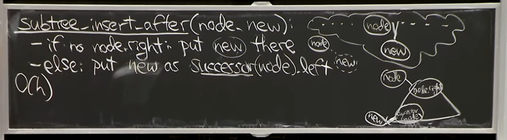
3.1 Subtree_insert_after(node_new)
Insert_after 의 경우는 traversal order에 따라 노드의 오른쪽이 비어있다면 그곳에 삽입, 그렇지 않으면 Successor 노드를 찾아서 왼쪽 노드를 리턴해서 다시 Insert_after를 재귀적으로 합니다. Time Complexity로는 node.right는 O(1), Successor의 경우는 O(h)가 되겠습니다.
Reference. MIT 6.006 Introduction to Algorithms, Spring 2020
3.2 Examples for Subtree_insert_after
Reference. MIT 6.006 Introduction to Algorithms, Spring 2020
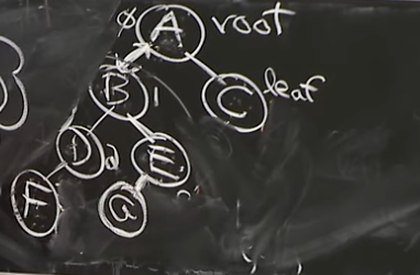
- Case 1: Insert G before E
- if Insert Left Child → Empty → Stick it there
- else Insert Right Child → Empty → Stick it there
Reference. MIT 6.006 Introduction to Algorithms, Spring 2020
-
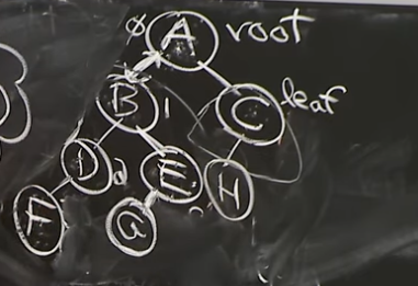
Case 2: Insert H after A
Reference. MIT 6.006 Introduction to Algorithms, Spring 2020
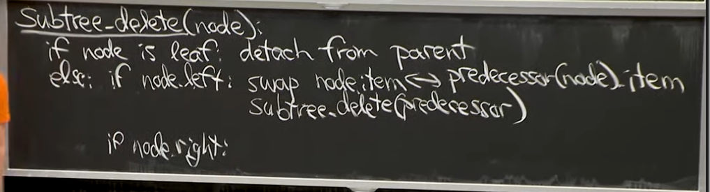
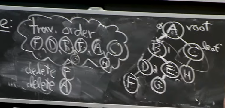
3.3 Subtree_delete(node)
Delete operation 에서는 “Predecessor Node와 Swapping”한다는 아이디어를 이용해서 지우면 되겠습니다.
Delete의 경우는 노드가 Leaf인 경우 바로 제거하면 되고, 노드의 왼쪽이 있는 경우는 Predecessor 노드를 찾아서 Swapping한 후 Leaf노드를 찾을 때 까지 이를 반복합니다. 결국 트리를 밑으로 내려가게 돼, Time Complexity는 O(h)가 되겠습니다.
Reference. MIT 6.006 Introduction to Algorithms, Spring 2020
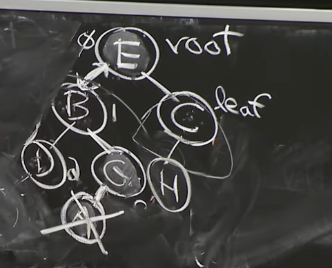
3.4 Examples for Subtree_delete
Reference. MIT 6.006 Introduction to Algorithms, Spring 2020
-
Case 1 Delete F: Leaf! Erase it.
Reference. MIT 6.006 Introduction to Algorithms, Spring 2020
-
Case 2 Delete A: Swap Predecessor(Node) and Erase Predecessor
Reference. MIT 6.006 Introduction to Algorithms, Spring 2020
4. Set and Sequence interface using Binary Tree
이제 Binary Tree data structure에 대해서 알아봤으니 Set / Sequence Interface에 대해서 알아볼 차례입니다.
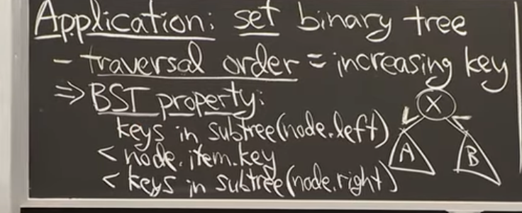
4.1 Set Binary Tree, subtree_find(node, k)
강의에서는 Set Binary Tree의 경우 Traversal order대로 item의 key를 늘리면서 간다고 설명합니다. Set Binary Tree의 경우에는 Binary Search Tree(BST)와 같은 구조가 될 겁니다.
Reference. MIT 6.006 Introduction to Algorithms, Spring 2020
그렇다면 Interface에서 중요한 find(k) operation을 확인해봐야겠죠. Set Binary Tree는 아래와 같을 수 있겠죠?
Reference. MIT 6.006 Introduction to Algorithms, Spring 2020
Find는 어렵지 않습니다. 처음에 Set Binary Tree 의 경우 Traversal order대로 item의 key를 늘리면서 간다고 언급했으니, k 번째 Node를 찾고 싶으면 k번째 Node의 key와 비교해서 작으면 왼쪽으로, 크면 오른쪽으로 가면 됩니다. 당연히, Time complexity는 O(h)가 될 겁니다.
subtree_find(node, k):
- if node is None: return
- if k < node.item key: recurse on node.left
- if = : return node
- if > : recurse on node.right
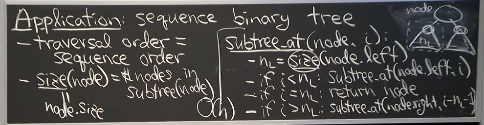
4.2 Sequence Binary Tree, subtree_find(node, k)
그럼 Sequence의 경우는, Sequence order는 Traversal order를 따라 갑니다.
Reference. MIT 6.006 Introduction to Algorithms, Spring 2020
그럼, key가 없는 Sequence는 어떻게 해야할까요? 여기서 “Sequence Augmentation”라는 개념이 등장합니다. 각 노드마다 한 가지 정보를 더 가지고 있는데, 그게 바로 Size 입니다.
4.3 Sequence Augmentation
참고로 “Size”는 index 가 아닙니다! Index의 경우 중간에 삽입/삭제가 생기는 경우 이후 index를 모두 바꿔야하는 추가적인 작업이 있지만, Size, 즉 해당 노드를 Root로 하는 Subtree의 Node의 개수를 각각의 노드가 가지고 있다면 Find operation은 O(h)의 Time complexity를 가질 수 있을 겁니다. (만약 size를 저장하지 않으면 Recursive를 사용해야돼, O(n)이 필요할 겁니다.)
Reference. MIT 6.006 Introduction to Algorithms, Spring 2020
그러면 Sequence Augmentation은 Leaf 노드를 삽입/삭제 한다면 O(h) ancestors에 업데이트 해줘야 합니다.
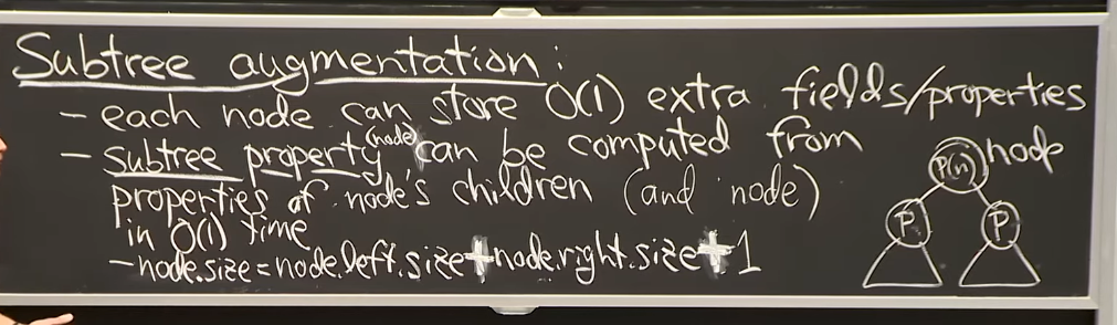
4.4 Subtree properties
Size 이외에도 매 노드마다 그 노드의 Subtree의 Sum, Product, Min, Max와 같은 Feature를 Subtree properties라고 부르겠습니다. Node의 index와 depth는 Subtree properties가 아닙니다.
강의에서는 “property to be local to a subtree vs global properties(index)” 라며 index를 global properties라고 언급하며 넘어갑니다.
5. AVL Tree
그런데, 아직 Time Complexity에서 O(h)라고 하지 O(log N)이라고 말하진 않습니다. 그 이유는 Tree에 데이터를 삽입/삭제를 하다보면 아래와 같은 “Unbalancing Binary Tree”를 만날 수 있기 입니다.
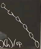
Worst case of binary tree, linear tree (Reference. MIT 6.006 Introduction to Algorithms, Spring 2020)
Balanced binary tree, $h = O(log n)$ 을 만들기 위해 등장하는 개념이 그래서 바로 “Rotate”와 “Height Balanced”입니다.
Reference. MIT 6.006 Introduction to Algorithms, Spring 2020
5.1 Rotate
Rotate Operation하기 이전에 먼저 짚고 넘어가야하는 부분이 있습니다. Binary Tree data structure의 Operation을 만들어 놓고, 이를 훼손하면 사용하기가 힘들겠죠? 그래서 “Rebalencing a tree, at the same time it should not change the data that’s represented by the tree, traversal order.” 이전에 언급했다시피, “Traversal order”를 훼손하지 않는 방향으로 Rotate를 하는 방법을 고안합니다.
Rotation Operation은 아래 그림을 보고 생각해보시죠! 매 Rotation시 A, B, C subtree의 Augmentation은 바뀌지 않지만, x와 y의 경우에는 업데이트를 해줘야겠습니다.
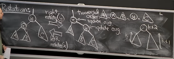
We will need to update h ancestor for augmentations, which is locally O(1) time, because subtree x changed when left rotate. In above picture, triangle means these operations preserve traversal order. (Reference. MIT 6.006 Introduction to Algorithms, Spring 2020)
5.2 AVL Tree
AVL Tree (named after inventors Adelson-Velsky and Landis는 그래서 이 Rotate Operation을 이용한 “Height Balanced”(AVL Property라고도 부릅니다) 를 가집니다. 여기서 Skew 란 오른쪽 subtree의 height와 왼쪽 subtree의 차이를 의미 합니다.
그럼 이 AVL Tree가 저희가 목표했던 $O(logn)$을 왜 가질 수 있는지 우선 증명해봐야겠죠?
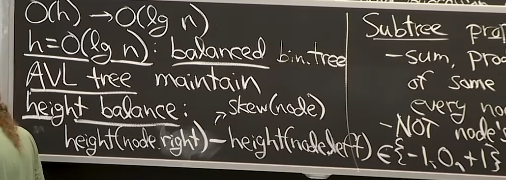
“Height Balenced” called the AVL Property. Let skew of a node be the height of its right subtree minus that of its left subtree(Reference. MIT 6.006 Introduction to Algorithms, Spring 2020)
아래 증명과정을 정리해봤습니다. N은 X 노드의 Size이며 h는 height를 의미합니다.
\[\begin{aligned} N_h &= N_{h-1} + N_{h-2} + 1 \\ &\geq N_{h-2} + N_{h-2} = 2 \cdot N_{h-2} = 2^{h/2}\\ &\rightarrow h \leq 2logn \end{aligned}\]
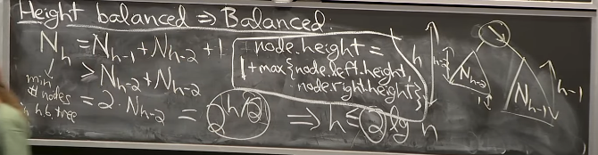
Why Height balanced’s h is logn? (Reference. MIT 6.006 Introduction to Algorithms, Spring 2020)
5.4 Examples for Balance in AVL Tree
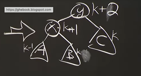
그럼 증명을 마쳤으니, Balance을 하는 예시를 들어보겠습니다. 가장 작은 Unbalance라고 가정한다면, Skew는 항상 +2와 -2가 될겁니다($\text{skew} \in {+2,-2}$). 화살표는 Unbalance하다고 생각하시면 됩니다.
- Consider lowest unbalanced node x, $\text{skew} \in {+2,-2}$
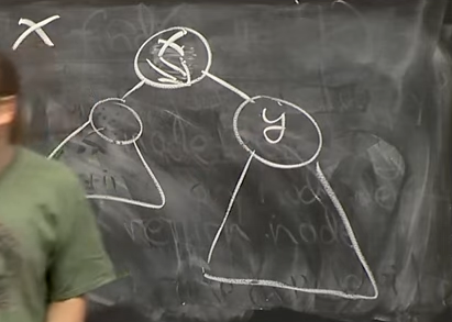
Reference. MIT 6.006 Introduction to Algorithms, Spring 2020
그 경우에 위 그림에서 y 노드의 skew의 경우를 다음 세가지로 나눌 수 있습니다. 1, 2번의 경우는 이해가 어렵지 않지만, 3번의 경우는 기억하고 넘어가시면 좋다고 합니다.
-
#1 Case 1 skew(y) = 1
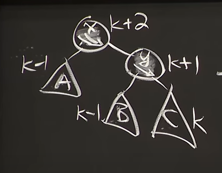
Reference. MIT 6.006 Introduction to Algorithms, Spring 2020
-
Balanced(Left Rotate $x$)
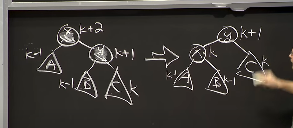
Reference. MIT 6.006 Introduction to Algorithms, Spring 2020
-
-
#2 Case 2 skew(y) = 0
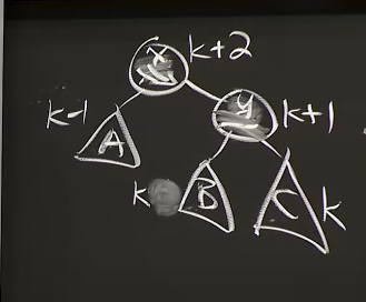
Reference. MIT 6.006 Introduction to Algorithms, Spring 2020
-
Balanced(Left Rotate $x$)
Reference. MIT 6.006 Introduction to Algorithms, Spring 2020
-
-
[NEED TO MEMORIZE] #3 Case 3 skew(z) = -1
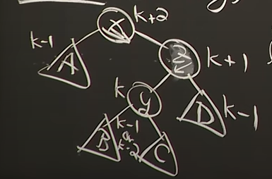
Reference. MIT 6.006 Introduction to Algorithms, Spring 2020
-
Balanced
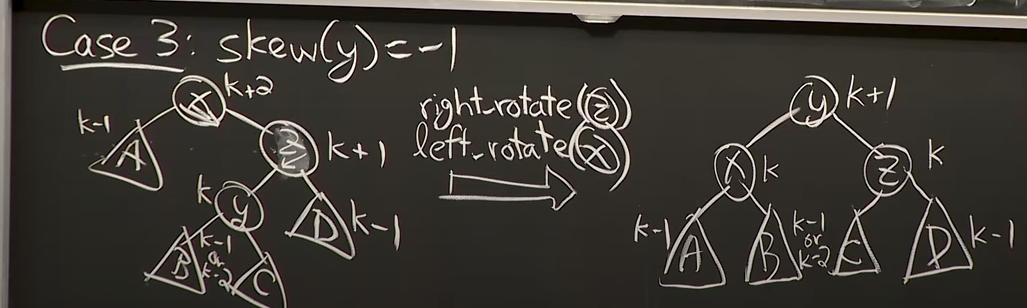
Reference. MIT 6.006 Introduction to Algorithms, Spring 2020
-
위의 예시에서 보면, “Check the Parent Node” 부모 노드를 확인해서 Unbalance 하다면, Balancing을 하면서 Node를 올라가면 Augmentation과 Balance를 height 만큼의 operation($O(logn)$)으로 가질 수 있습니다. 강의에서는 다음과 같이 말합니다.
“Maybe Parent is out of balance, and we just keep walking up the node, and also maintain all the augmentations as we go.
This keeps track of heights and subtree size. And **after order h(= O(logn)) operations,**
we have restored **height balanced property**.”
AVL Tree에 대해서 Insert/Delete 그리고 Balancing이 보고 싶으시다면 이 링크를 타시면 되겠습니다.
Binary Tree의 개념은 여기까지 입니다(강의에서는 Binary Tree, Part1 - Part2: AVL까지 입니다). 추가적으로 Priority queue interface에서 사용하는 Binary Heap이 Complete Binary Tree의 구조를 띄고 있어, 짚고 넘어가볼까 합니다.
6. Priority queue interface(subset of Set)
6.1 Operations
Priority queue interface
------------------------
- build(x): init to items in x
- insert(x): add item x
- delete_max(): delete & return max-key item
- find_max(): return max-key item
Priority queue interface(우선 순위 큐)는 FIFO(First Input First Out)을 가지면서 Priority를 가지는 Set Interface입니다. 이 Interface에서 중요한 Operation은 build, insert, 그리고 delete_max 입니다. delete_max를 보니 Sorting을 할 수 있겠다는 생각이 들 수 있습니다.
Reference. MIT 6.006 Introduction to Algorithms, Spring 2020
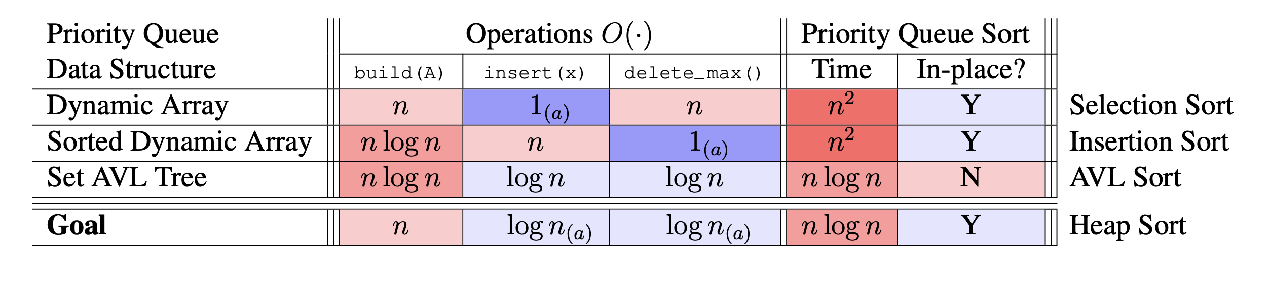
우선 Data Structrue에 대해 먼저 이야기해보면, 고려해 볼 수 있는 경우는 Set AVL Tree, Array, Sorted Array가 있고 각 Data structure의 필요한 Operation의 Time complexity는 아래와 같이 볼 수 있습니다.
- Array: Insert O(1) amortized, delete_max O(n)
- Sorted array: Insert O(n), delete_max O(1) amortized
- Set AVL Tree: Insert O(log n) → delete_max O(1) augment(O(1)) → find_max by storing in every node the maximum key item)
6.2 Priority queue sort
Data Structure와 더불어, Max Operation을 이용해서 사용할 수 있는 Sorting인 Priority queue sort가 있을 수 있습니다. Priority Queue Sort의 Operation은 어떻게 해야 할 까요?
- build(A): insert(x) for x in A
- repeatedly delete_max()
Priority Queue Sort를 위해서는 Data Structure와 동일하게 Set AVL Tree, Array, Sorted Array를 이용할 수 있겠습니다. 각각 시간복잡도를 구해보면, 다음과 같습니다.
- Array: Selection Sort $O(n^2)$
- Sorted array: Insertion Sort $O(n^2)$
- Set AVL Tree: build $O(nlogn)$ → delete_max O(1) (augmentation Max 로 $O(1)$, find_max by storing in every node the maximum key item)
이 외에도 Priority Queue Sort를 Merge Sort를 이용해도 되겠습니다. 하지만 $O(nlogn)$의 Time complexity를 가지는 Merge Sort와 AVL Sort는 In-place가 아니라는 부분이 있습니다(Merge sort and Set AVL tree sort are not in-place!).
여기서 Binary Heap이 나오는 이유를 크게 “Build O(n) & main reason is in-place sorting algorithm”로 설명합니다. Simplified version of Set AVL 인 Binary Heap에 대해서 시작해보겠습니다.
7. Binary Heap, Complete binary tree
7.1 Definition
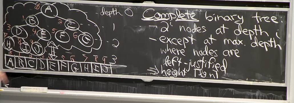
이 그림을 보시면 알 수 있듯이, Tree의 구조를 Array에 그대로 담을 수가 있습니다(Reference. MIT 6.006 Introduction to Algorithms, Spring 2020)
Binary Heap은 Complete binary tree(완전 이진 트리)의 구조를 가지며 다음과 같은 특성들을 가집니다.
- For every complete binary tree, there’s a unique array!
- No rotations necessary in heaps because complete binary tree
- $height= log(n)$
- We don’t need to store left/right and parent pointers, just store array
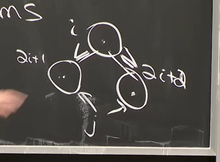
-
Implicit data structure: no pointers, just array of n items. → Tree is our thought! Only array
\[\begin{aligned} &left(i)=2i+1 \\ &right(i)=2i+2 \\ &parent(i) = trunc\big(\dfrac{i-1}{2}\big) \end{aligned}\]
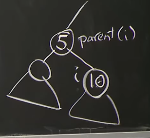
7.2 Max-Heap Property in Binary Heap Q
Binary Heap의 특징 중에 하나는 바로 Max-Heap Property입니다. Max-Heap Property란 Array representing complete binary tree where every node I satisfies,
\[i: Q[i]\geq Q[i]\ for\ j \in \{left(i),\ right(i)\},\]- Lemma: $Q[i] \geq Q[j]$ for node j in subtree(i)
Reference. MIT 6.006 Introduction to Algorithms, Spring 2020
간단히 말하면 부모노드가 자식노드 보다 크다는 것을 말합니다. Data structrion의 정의를 봤으니 Operation인 Insert와 Delete를 볼 차례 입니다.
7.2 Insert
Reference. MIT 6.006 Introduction to Algorithms, Spring 2020
위의 그림과 같이 10을 Heap에 넣을 것이라고 가정해 봅시다. 그러면 Insert operation은 Insert_last와 max_heapify_up(max_heapify_up은 stack overflow에서 siftUp라고도 불리더군요)으로 이뤄집니다.
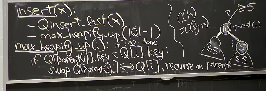
Reference. MIT 6.006 Introduction to Algorithms, Spring 2020
부모 노드보다 키값이 작다면 Swap을 계속 반복하게 되며, 그렇다면 O(log(N))만큼의 Time Complexity를 가질 겁니다.
7.3 Delete
Delete의 경우에는 어떨까요? Leaf 노드의 경우 간단히 삭제하면 되니, 부모노드의 경우를 살펴보겠습니다.
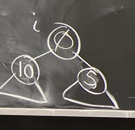
Reference. MIT 6.006 Introduction to Algorithms, Spring 2020
위 그림 처럼 부모노드를 삭제하고 그 자리가 비게되면, Insert와 비슷하게 delete_max와 max_heapify_down을 반복해서 Leaf노드까지 내려가게 됩니다. delete_max는 왼쪽/오른쪽 노드를 비교해서 큰 노드와 Swap하는 것을 말합니다.
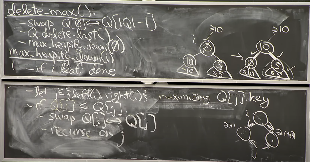
Reference. MIT 6.006 Introduction to Algorithms, Spring 2020
Delete Operation도 그럼 Time Complexity가 $O(logN)$이 되겠네요.
그럼 Heap Sort는 어떻게 짜야할까요? 데이터가 N개가 있으면 Insert로 Binary Heap을 만든 후, delete_max로 데이터를 하나씩 빼내면 Priority Queue sort가 될 수 있겠습니다.
7.4 Inplace
그렇다면 왜 Heap Sort가 In-place가 될까요? 아래 그림처럼 Array A를 Priority Queue sort하려면 왼쪽 데이터부터 차례로 Insert하다가 Binary Heap이 모두 build가 되면 delete_max를 하면 됩니다. 추가적인 메모리가 필요없는 걸 볼 수 있습니다.
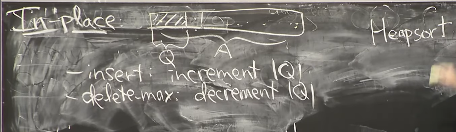
Reference. MIT 6.006 Introduction to Algorithms, Spring 2020
7.5 Build
그럼 Build는 왜 $O(n)$ 일까요? 분명 Insert를 Root에서 부터 한다고 생각하면, max_heapify_up을 하게 되면 $\sum depth(i) = \sum log\ i = O(nlogn)$ 인데 말입니다. 방법은 의외로 간단합니다.
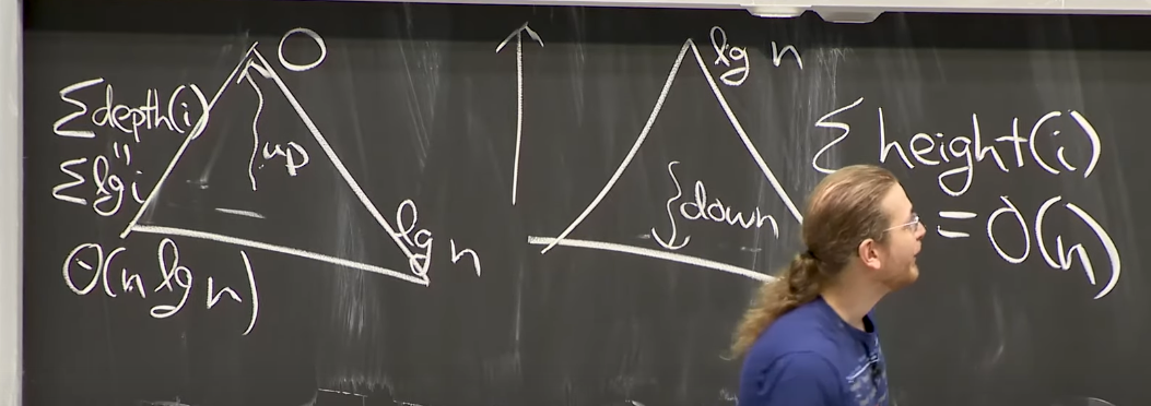
Reference. MIT 6.006 Introduction to Algorithms, Spring 2020
밑에서 부터 시작한다고 생각하시면 됩니다. 그러면 Insert를 하고 max_heapify_down을 하게되면 $\sum height(i)=O(n)$ 을 가질 수 있을 겁니다. 직관적으로 봤을때, 가장 연산이 많이 드는 Leaf노드에서 heapify_up 보다 heapify_down을 하게 되면 $O(log\ n)$ 이 $O(1)$이 되니, build의 Time complexity는 $O(n)$이 될 겁니다. 수식적으로 보고 싶으시다면 이 링크에 들어가서 확인하시면 되겠습니다.
여기까지 Binary Tree, Binary Tree for Set Interface(Binary Search Tree), Binary Tree for Sequence Interface, AVL, 그리고 Heap Tree까지 살펴봤습니다. 이외에도 B Tree와 B++ Tree도 Binary Tree의 연장선으로 보이는데, 이에 대해서는 추후 이야기하도록 하겠습니다.