All contents is arranged from CS224N contents. Please see the details to the CS224N!
1. Intro
How can we predict a center word from the surrounding context in terms of word vectors?
One approach is If we treat {“The”, “cat”, ’over”, “the’, “puddle”} as a context and from these words, it will be able to predict or generate the center word “jumped”.
We defines as below,
- $x^{(c)}$ : The input one-hot vectors or context
- $y^{(c)}$ : The output, we just call this y which is the one-hot vector of the known center word.
- $w_i$: Word i from vocabulary V
- $\nu \in \mathbb{R}^{n \times \lvert V\lvert}$ : Input word matrix
- ${v}_i$: i-th column of $\nu$ , the input vector representation of word $w_i$
- $u \in \mathbb{R}^{\lvert V\lvert\times n}$ : Output word matrix
- $u_i$: i-th row of $u$, the output vector representation of word $w_i$
- Note that we do in fact learn two vectors for every word $w_i$
- n is an arbitrary size that defines the size of our embedding space
- ${v}_i$: input word vector, when the word is in the context
- $u_i$: output word vector, when the word is in the center
2. Steps
-
Generate our one-hot word vectors for the input context of size
$m: (x^{c-m}, \dots, x^{c-1}, x^{c+1}, \dots, x^{c+m}) \in \mathbb{R}^{\lvert V\lvert}$
-
Get Embedded word vectors for the context
$v_{c-m} = \nu x^{c-m}, v_{c-m+1} = \nu x^{c-m+1}, \dots, v_{c+m} = \nu x^{c+m} \in \mathbb{R}^n$
-
Average these vectors to get
$\hat{v} = \dfrac{v_{c-m}+v_{c-m+1}+\dots+v_{c+m}}{2m} \in \mathbb{R}^n$
-
Generate a score vector $z = u\hat{v} \in \mathbb{R}^{\lvert V\lvert}$. As the dot product of similar vectors is higher, it will push similar words close to each other in order to achieve a high score.
-
Turn the scores into probabilities $\hat{y} = softmax(x) \in \mathbb{R}^{\lvert V\lvert}$
\[i\small{-}th \ component \ is \ \dfrac { e^{\hat{y}_i} } { \displaystyle\sum_{k=1}^{\lvert V\lvert}e^{\hat{y}_k} }\]-
Exponentiate is to make positive, and dividing by $\displaystyle\sum_{k=1}^{\lvert V\lvert}e^{\hat{y}_k}$ normalizes
the vector $(\textstyle\sum_{k=1}^{n}\hat y_k=1)$ to give probability
-
-
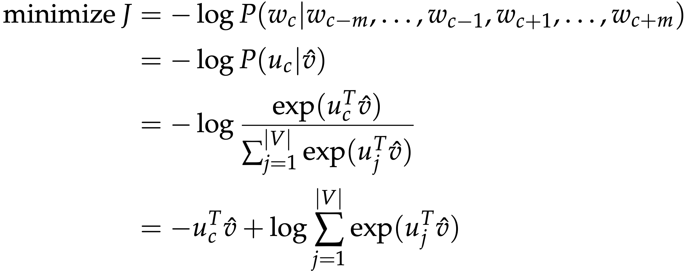
We desire our probabilities generated, $\hat{y}\in \mathbb{R}^{\lvert V\lvert}$, to match the true probabilities, $\text{y}\in \mathbb{R}^{\lvert V\lvert}$, which also happens to be the one-hot vector of the actual word.
-
We use a popular choice of distance/loss measure, cross entropy $H(\hat{y},y)$.
$H(\hat{y}, y) = \displaystyle\sum_{j=1}^{\lvert V\lvert}y_jlog(\hat{y}_j)$
-
Because y is one-hot vector, thus the above loss simplifies to simply:
$H(\hat{y}, y) = y_jlog(\hat{y}_j)$
- In this formulation, c is the index where the correct word’s one-hot vector is 1. We can now consider the case where our prediction was perfect and thus $\hat{y}$c = 1. We can then calculate H($\hat{y}$, y) =-1 log(1) = 0. Thus, for a perfect prediction, we face no penalty or loss.
Reference. cs224n-2019-notes01-wordvecs1
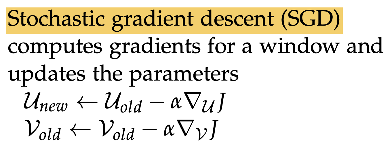
- We use stochastic gradient descent to update all relevant word vectors $u_c$ and $v_j$.
Reference. cs224n-2019-notes01-wordvecs1