Evaluation of Word Vectors

All contents is arranged from CS224N contents. Please see the details to the CS224N!

1. Intrinsic and Extrinsic Evaluation

$\checkmark$ Intrinsic evaluation

• Evaluation on a specific, intermediate task
• Fast to compute performance
• Helps understand subsystem
• Needs positive correlation with real task to determine usefulness
• To train a machine learning system
  1. Takes words as inputs
  2. Converts them to word vectors
  3. Uses word vectors as inputs for an elaborate machine learning system
  4. Maps the output word vectors by this system back to natural language words
  5. Produces words as answers

$\checkmark$ Extrinsic evaluation

• Is the evaluation on a real task
• Can be slow to compute performance
• Unclear if subsystem is the problem, other subsystems, or internal interactions
• If replacing subsystem improves performance, the change is likely good

2. Intrinsic Example: Word Vector Analogies

$\checkmark$ a:b :: c:?

• This intrinsic evaluation system then identifies the word vector which maximizes the cosine similarity

  \[d = \underset{i}{argmax} \dfrac{(x_b-x_a+x_c)^T x_i}{\lvert\lvert x_b-x_a+x_c \lvert\lvert}\]
• Ideally, we want $x_b − x_a = x_d − x_c$ (For instance, queen – king = actress – actor).
• We identify the vector xd which maximizes the normalized dot-product between the two word vectors (i.e. cosine similarity).

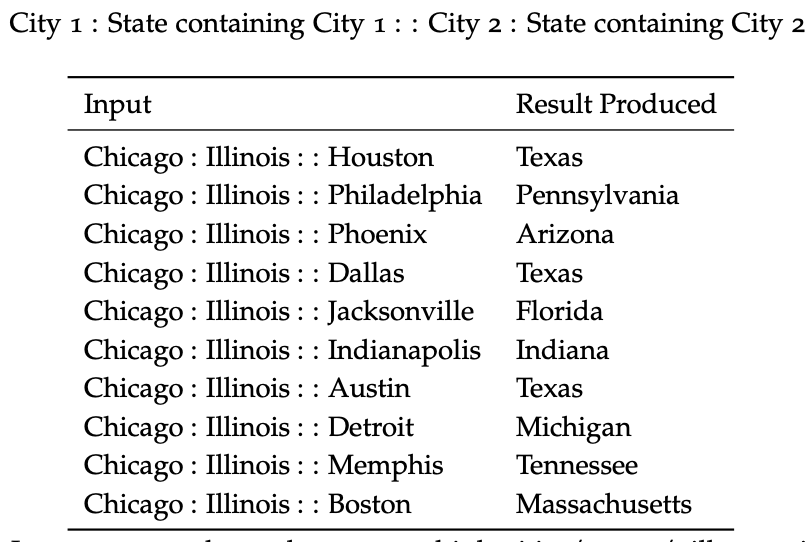
• Semantic word vector analogies (intrinsic evaluation) that may suffer from different cities having the same name

  

  Reference. cs224n-2019-notes01-wordvecs1

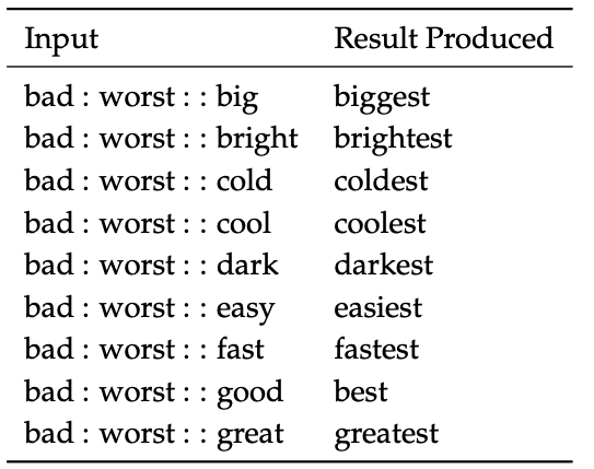
• Syntactic word vector analogies (intrinsic evaluation) that test the notion of superlative adjectives.

  

  Reference. cs224n-2019-notes01-wordvecs1

$\checkmark$ Analogy Evaluation Tuning Example

• Some of the hyperparameters in word vector embedding techniques (such as Word2Vec and GloVe) that can be tuned using an intrinsic evaluation system (such as an analogy completion system)
  • Dimension of word vectors
  • Corpus size
  • Corpus souce/type
  • Context window size
  • Context symmetry

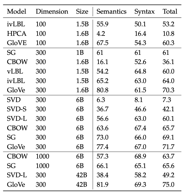
• Here we compare the performance of different models under the use of different hyperparameters and datasets.

  

  Reference. cs224n-2019-notes01-wordvecs1

  • Inspecting the above table, we can make 3 primary observations:

    • Performance is heavily dependent on the model used for word embedding

      This is an expected result since different methods try embedding words to vectors using fundamentally different properties (such as co-occurrence count, singular vectors, etc.)

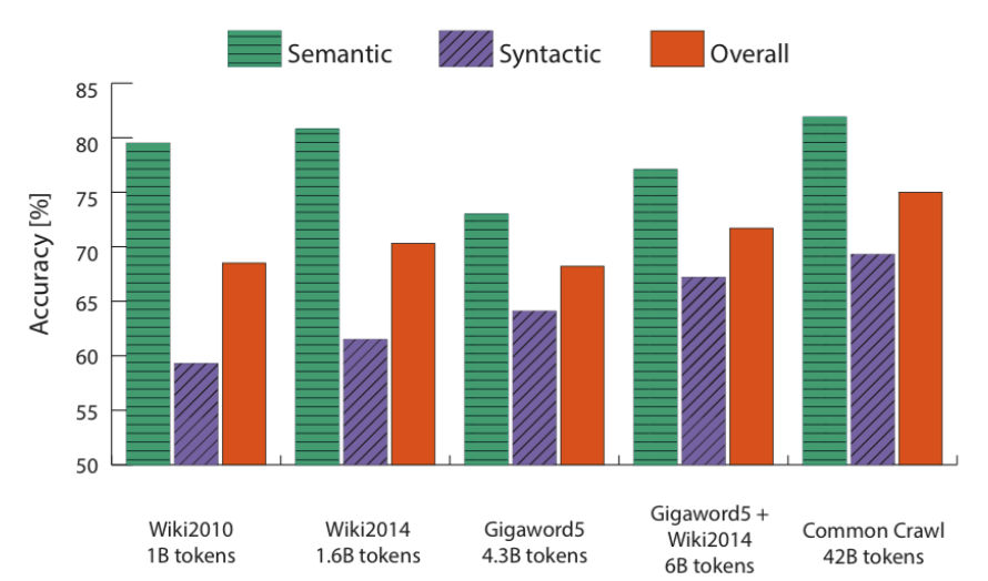
    • Performance increases with larger corpus sizes

      This happens because of the experience an embedding technique gains with more examples it sees. For instance, an analogy completion example will produce incorrect results if it has not encountered the test words previously.

    • Performance is lower for extremely low dimensional word vectors

      Lower dimensional word vectors are not able to capture the different meanings of the different words in the corpus. This can be viewed as a high bias problem where our model complexity is too low. For instance, let us consider the words “king”, “queen”, “man”, “woman”. Intuitively, we would need to use two dimensions such as “gender” and “leadership” to encode these into 2-bit word vectors. Any lower would fail to capture semantic differences between the four words.

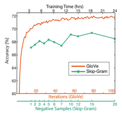
  • Below Figure demonstrates how accuracy has been shown to improve with larger corpus.

    

    Reference. cs224n-2019-notes01-wordvecs1

  • Below Figure demonstrates how other hyperparameters have been shown to affect the accuracies using GloVe.

    

    Reference. cs224n-2019-notes01-wordvecs1

    Figure. We see how accuracies vary with vector dimension and context window size for GloVe

  • Implementation Tip

    1. A window size of 8 around each center word typically works well for GloVe embeddings.

       

       Reference. cs224n-2019-notes01-wordvecs1

    2. Extremely high dimensional vectors

       Intuitively, it would seem that these vectors would capture noise in the corpus that doesn’t allow generalization, i.e. resulting in high variance, but Yin et al. show in On the Dimensionality of Word Embedding that skip-gram and GloVe are robust to this over-fitting.

$\checkmark$ Correlation Evaluation

Another simple way to evaluate the quality of word vectors is by asking humans to assess the similarity between two words on a fixed scale (say 0-10) and then comparing this with the cosine similarity between the corresponding word vectors.

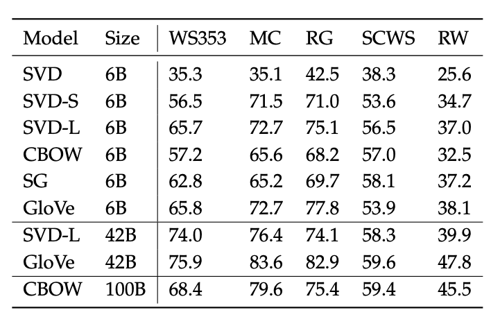
Table. Here we see the correlations between of word vector similarities using different embedding techniques with different human judgment datasets, Reference. cs224n-2019-notes01-wordvecs1

$\checkmark$ Dealing with Ambiguity

• For instance, “run” is both a noun and a verb and is used and interpreted differently based on the context. Improving Word Representations Via Global Context And Multiple Word Prototypes (Huang et al, 2012)

• The essence of the method

  1. Gather fixed size context windows of all occurrences of the word (for instance, 5 before and 5 after)
  2. Each context is represented by a weighted average of the context words’ vectors (using idf-weighting)
  3. Apply spherical k-means to cluster these context representations.
  4. Finally, each word occurrence is re-labeled to its associated cluster and is used to train the word representation for that cluster.

3. Training for Extrinsic Tasks

$\checkmark$ In named-entity recognition (NER)

• Given a context and a central word, we want to classify the central word to be one of many classes.

• For the input, “Jim bought 300 shares of Acme Corp. in 2006”, we would like a classified output

  \[[Jim]_{Person}\ bought\ 300\ shares\ of\ [Acme\ Corp.]_{Organization}\ in\ [2006]_{Time}.\]

• For such problems, we typically begin with a training set of the form

  \[\{x^{(i)},y{(i)}\}^N_1\]

  where $x^{(i)}$ is a d-dimensional word vector generated by some word embedding technique and $y^{(i)}$ is a C-dimensional one-hot vector which indicates the labels we wish to eventually predict(sentiments, other words, named entities, buy/sell decisions, etc.).

  

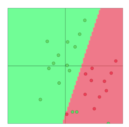
  We can classify word vectors using simple linear decision boundaries such as the one shown here (2-D word vectors) using techniques such as logistic regression and SVMs, Reference. cs224n-2019-notes01-wordvecs1

• In typical machine learning tasks, we usually hold input data and target labels fixed and train weights using optimization techniques (such as gradient descent, L-BFGS, Newton’s method, etc.)
• we introduce the idea of retraining the input word vectors when we train for extrinsic tasks

$\checkmark$ Retraining Word Vectors

In many cases, these pre-trained word vectors are a good proxy for optimal word vectors for the extrinsic task and they perform well at the extrinsic task. However, it is also possible that the pre-trained word vectors could be trained further (i.e. retrained) using the extrin- sic task this time to perform better. However, retraining word vectors can be risky.

If we retrain word vectors using the extrinsic task, we need to en- sure that the training set is large enough to cover most words from the vocabulary. This is because Word2Vec or GloVe produce semanti- cally related words to be located in the same part of the word space. When we retrain these words over a small set of the vocabulary, these words are shifted in the word space and as a result, the performance over the final task could actually reduce. Let us explore this idea further using an example. Consider the pretrained vectors to be in a two dimensional space as shown in Figure.

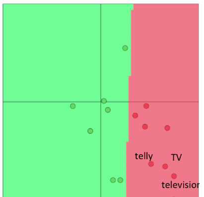
Here, we see that the words "Telly", "TV", and "Television" are clas- sified correctly before retraining. "Telly" and "TV" are present in the extrinsic task training set while "Television" is only present in the test set, Reference. cs224n-2019-notes01-wordvecs1

Here, we see that the word vectors are classified correctly on some extrinsic classification task. Now, if we retrain only two of those vectors because of a limited training set size, then we see in below Figure that one of the words gets misclassified because the boundary shifts as a result of word vector updates.

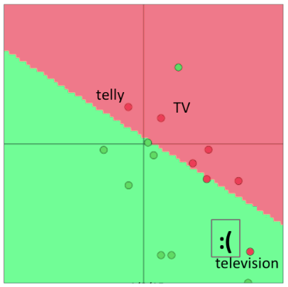
Here, we see that the words "Telly" and "TV" are classified correctly after training, but "Television" is not since it was not present in the training set, Reference. cs224n-2019-notes01-wordvecs1

Thus, word vectors should not be retrained if the training data set is small. If the training set is large, retraining may improve performance.

4. Softmax Classification and Regularization

• Softmax classification function

  \[p(y_j=1\lvert x) = \dfrac{exp(W_j \cdot x)}{\sum_{c=1}^C exp(W_c \cdot x)}\]

• The probability of word vector x being in class j. Using the Cross-entropy loss function, we calculate the loss of such a training example as:

  \[-\displaystyle\sum_{j=1}^C y_j log(p(y=j=1\lvert x)) = -\displaystyle\sum_{j=1}^C y_j log (\dfrac{exp(W_j \cdot x)}{\sum_{c=1}^C exp(W_c \cdot x)})\]

• Of course, the above summation will be a sum over (C − 1) zero values since $y_j$ is 1 only at a single index (at least for now) implying that x belongs to only 1 correct class. Thus, let us define k to be the index of the correct class. Thus, we can now simplify our loss to be:

  \[\dfrac{exp(W_j \cdot x)}{\sum_{c=1}^C exp(W_c \cdot x)}\]

• We can then extend the above loss to a dataset of N points:

  \[-\displaystyle\sum_{i=1}^N log(\dfrac{exp(W_{k(i)} \cdot x^{(i)})}{\sum_{c=1}^C exp(W_c \cdot x^{(i)})} )\]
• The only difference above is that $k(i)$ is now a function that returns the correct class index for example $x^{(i)}$.

• [TODO] NOT UNDERSTANDING YET

  Let us now try to estimate the number of parameters that would be updated if we consider training both, model weights (W), as well word vectors (x). We know that a simple linear decision boundary would require a model that takes in at least on $d$ dimensional input word vector and produces a distribution over $C$ classes. Thus, to update the model weights, we would be updating $C \cdot d$ parameters. If we update the word vectors for every word in the vocabulary $V$ as well, then we would be updating as many as $\lvert V \lvert$ word vectors, each of which is $d$-dimensional. Thus, the total number of parameters would be as many as $C \cdot d + \lvert V\lvert \cdot d$ for a simple linear classifier:

  \[\nabla_{\theta}J(\theta) = \begin{bmatrix} \nabla_{x_{(\cdot 1)}} \\ \vdots \\ \nabla_{x_{W_{\cdot d}}} \\ \nabla_{x_{aardvark}} \\ \vdots \\ \nabla_{x_{zebra}} \\ \end{bmatrix}\]

  This is an extremely large number of parameters considering how simple the model’s decision boundary is - such a large number of parameters is highly prone to overfitting.

  To reduce overfitting risk, we introduce a regularization term which poses the Bayesian belief that the parameters (θ) should be small is magnitude (i.e. close to zero):

  \[-\displaystyle\sum_{i=1}^N log(\dfrac{exp(W_{k(i)} \cdot x^{(i)})}{\sum_{c=1}^C exp(W_c \cdot x^{(i)})} ) + \lambda \displaystyle\sum_{k=1}^{C\cdot d + \lvert V \lvert \cdot d} \theta^2_k\]

  Minimizing the above cost function reduces the likelihood of the parameters taking on extremely large values just to fit the training set well and may improve generalization if the relative objective weight λ is tuned well. The idea of regularization becomes even more of a requirement once we explore more complex models (such as Neural Networks) which have far more parameters.

5. Window Classification

• Natural languages tend to use the same word for very different meanings and we typically need to know the context of the word usage to discriminate between meanings.

• For instance, if you were asked to explain to someone what “to sanction” meant, you would immediately realize that depending on the context “to sanction” could mean “to permit” or “to punish”.

• In most situations, we tend to use a sequence of words as input to the model. A sequence is a central word vector preceded and succeeded by context word vectors. The number of words in the context is also known as the context window size and varies depending on the problem being solved.

• Generally, narrower window sizes lead to better performance in syntactic tests while wider windows lead to better performance in semantic tests.

• In order to modify the previously discussed Softmax model to use windows of words for classification, we would simply substitute $x^{(i)}$ with $x_{window}^{(i)}$:

  \[x_{window}^{(i)} = \begin{bmatrix} x^{(i-2)} \\ x^{(i-1)} \\ x^{(i)} \\ x^{(i+1)} \\ x^{(i+2)} \\ \end{bmatrix}\]

  As a result, when we evaluate the gradient of the loss with respect to the words, we will receive gradients for the word vectors:

  \[\delta_{window}^{(i)} = \begin{bmatrix} \nabla_x^{(i-2)} \\ \nabla_x^{(i-1)} \\ \nabla_x^{(i)} \\ \nabla_x^{(i+1)} \\ \nabla_x^{(i+2)} \\ \end{bmatrix}\]

  The gradient will of course need to be distributed to update the corresponding word vectors in implementation.

6. Non-linear Classifiers

We see in Figure 1 that a linear classifier mis- classifies many datapoints. Using a non-linear decision boundary as shown in Figure 2, we manage to classify all training points accu- rately. Although oversimplified, this is a classic case demonstrating the need for non-linear decision boundaries. In the next set of notes, we study neural networks as a class of non-linear models that have performed particularly well in deep learning application

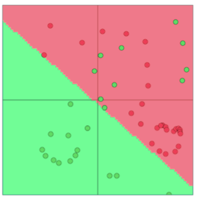
Here, we see that many examples are wrongly classified even though the best linear decision boundary is chosen. This is due linear decision boundaries have limited model capacity for this dataset, Reference. cs224n-2019-notes01-wordvecs1

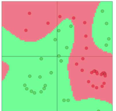
Here, we see that the non-linear decision boundary allows for much better classification of datapoints, Reference. cs224n-2019-notes01-wordvecs1