All contents is arranged from CS224N contents. Please see the details to the CS224N!
1. Intro
- In practice, hierarchical softmax tends to be better for infrequent words, while negative sampling works better for frequent words and lower-dimensional vectors.
- Hierarchical softmax uses a binary tree to represent all words in the vocabulary.
2. Real Contents from lecture
Mikolov et al. also present hierarchical softmax as a much more efficient alternative to the normal softmax. In practice, hierarchical softmax tends to be better for infrequent words, while negative sampling works better for frequent words and lower-dimensional vectors.
Hierarchical softmax uses a binary tree to represent all words in the vocabulary. Each leaf of the tree is a word, and there is a unique path from root to leaf. In this model, there is no output representation for words. Instead, each node of the graph (except the root and the leaves) is associated to a vector that the model is going to learn.
Reference. cs224n-2019-notes01-wordvecs1
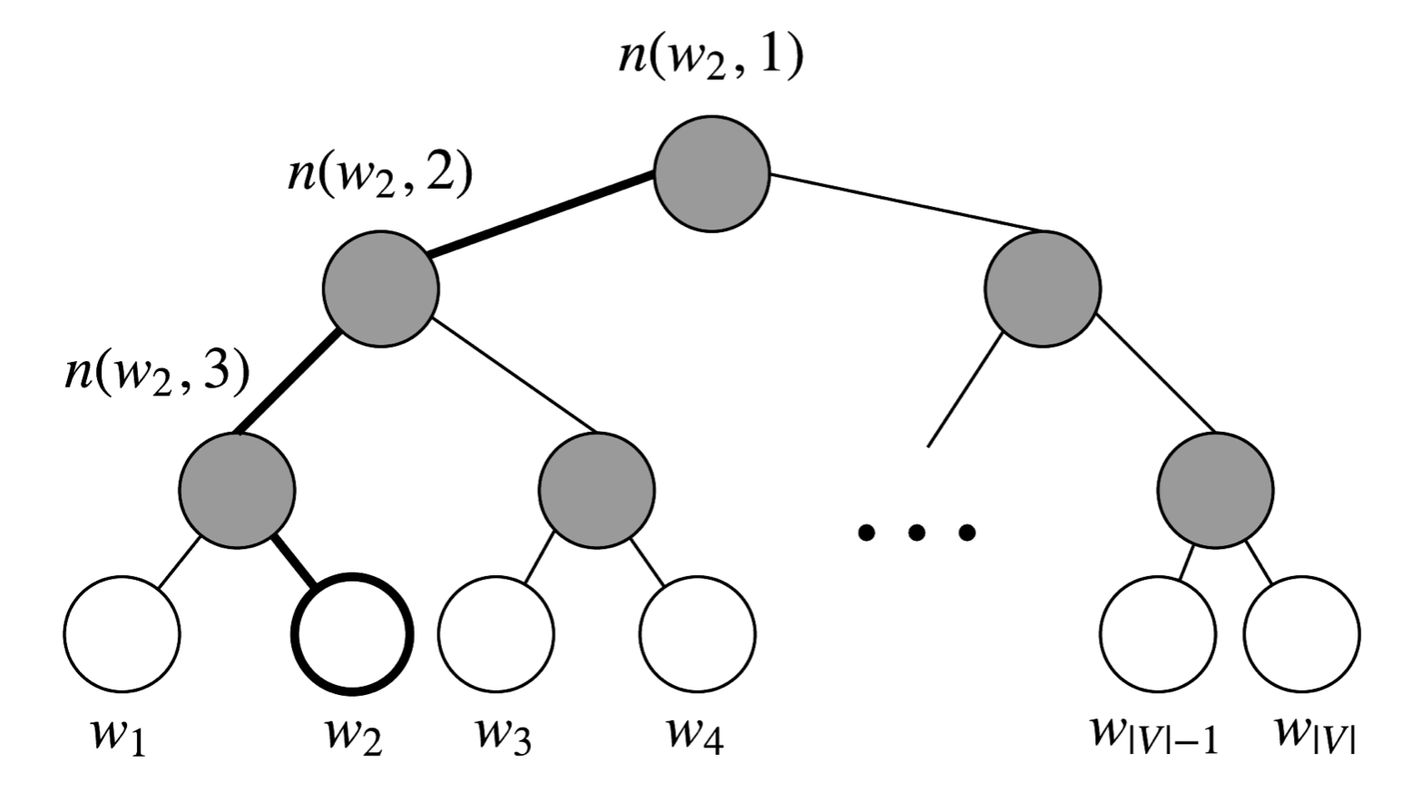
Figure is Binary tree for Hierarchical softmax, Hierarchical Softmax uses a binary tree where leaves are the words. The probability of a word being the output word is defined as the probability of a random walk from the root to that word’s leaf. Computational cost becomes $O(log(\lvert V\lvert ))$ instead of $O(\lvert V\lvert )$
In this model, the probability of a word w given a vector $w_i$, $P(w\lvert w_i)$, is equal to the probability of a random walk starting in the root and ending in the leaf node corresponding to w. The main advantage in computing the probability this way is that the cost is only $O(log(\lvert V\lvert ))$, corresponding to the length of the path.
Let’s introduce some notation. Let $L(w)$ be the number of nodes in the path from the root to the leaf $w$. For instance, $L(w_2)$ in Figure is 3. Let’s write $n(w, i)$ as the i-th node on this path with associated vector $v_{n(w,i)}$. So $n(w, 1)$ is the root, while $n(w, L(w))$ is the father of $w$. Now for each inner node $n$, we arbitrarily choose one of its children and call it $ch(n)$ (e.g. always the left node). Then, we can compute the probability as
\[P(w\lvert w_i) = \displaystyle\prod_{j=1}^{L(w)-1} \sigma([n(w, j+1)=ch(n(w, j))] \cdot v_{n(w,j)}^Tv_{w_i})\]where,
\[[x] = \begin{cases} 1 & \text{if } x \text{ is true} \\ -1 & \text{otherwise} \end{cases}\]and σ(·) is the sigmoid function. This formula is fairly dense, so let’s examine it more closely.
First, we are computing a product of terms based on the shape of the path from the root $n(w, 1)$ to the leaf $w$. If we assume $ch(n)$ is always the left node of $n$, then term $[n(w, j + 1) = ch(n(w, j))]$ returns 1 when the path goes left, and -1 if right.
Furthermore, the term $[n(w, j + 1) = ch(n(w, j))]$ provides normalization. At a node n, if we sum the probabilities for going to the left and right node, you can check that for any value of $v_n^T, \ v_{w_i}$
\[\sigma(v_n^Tv_{w_i}) + \sigma(-v_n^Tv_{w_i})=1\]The normalization also ensures that $∑\lvert V\lvert P(w\lvert w_i) = 1$, just as in w=1. Finally, we compare the similarity of our input vector $v_{w_i}$ to each the original softmax inner node vector $v^T$ using a dot product. Let’s run through an n(w, j) example. Taking $w_2$ in Figure, we must take two left edges and then a right edge to reach $w_2$ from the root, so
\[\begin{aligned} P(w_2\lvert w_i) &= p(n(w_2, 1), \text{left}) \cdot p(n(w_2, 2), \text{left}) \cdot p(n(w_2, 3), \text{right}) \\ &= \sigma(v_{n(w_2, 1)}^T v_{w_i}) \cdot \sigma(v_{n(w_2, 2)}^T v_{w_i}) \cdot \sigma(v_{n(w_2, 3)}^T v_{w_i}) \end{aligned}\]To train the model, our goal is still to minimize the negative log likelihood $-log P(w\lvert w_i )$. But instead of updating output vectors per word, we update the vectors of the nodes in the binary tree that are in the path from root to leaf node.
The speed of this method is determined by the way in which the binary tree is constructed and words are assigned to leaf nodes. Mikolov et al. use a binary Huffman tree, which assigns frequent words shorter paths in the tree.
3. Reference
- Korean Reference: https://wikidocs.net/22660
- Block Diagram: https://myndbook.com/view/4900
- Detail: [Rong, 2014] Rong, X. (2014). word2vec parameter learning explained. CoRR, abs/1411.2738.
- Hierarchical Softmax: [Mikolov et al., 2013] Mikolov, T., Chen, K., Corrado, G., and Dean, J. (2013). Efficient estimation of word representations in vector space. CoRR, abs/1301.3781.