Mathmatic for Stochastic Gradient Descent in Neural networks

All contents is arranged from CS224N contents. Please see the details to the CS224N!

1. Update equation

\[\theta^{new} = \theta^{old}-\alpha\nabla_{\theta}J(\theta),\ \alpha=step\ size\ or\ learning\ rate\]

For each parameter,

\[\theta^{new} = \theta^{old}-\alpha\dfrac{\partial J(\theta)}{\partial\theta_j^{old}}\]

2. Backpropagation algorithm, How to Compute $\nabla_{\theta}J(\theta)$?

1. Gradients

\[f(x)=x^3 \rightarrow \dfrac{df}{dx} = 3x^2\]

How much will the output change if we change the input a bit?

\[f(x) = f(x_1, x_2, \cdots, x_n) \rightarrow \dfrac{\partial f}{\partial x}=[\dfrac{\partial f}{\partial x_1}, \dfrac{\partial f}{\partial x_2}, \cdots, \dfrac{\partial f}{\partial x_n}]\]

2. Jacobian Matrix: Generalization of the Gradient

Approximate non-linear transform in the small scale(small $\partial x$) to linear transform. It’s Jacobian $m \times n$ matrix of partial derivatives.

\[\dfrac{\partial f}{\partial x} = \begin{bmatrix} \dfrac{\partial f_1}{\partial x_1} & \cdots & \dfrac{\partial f_1}{\partial x_n}\\ \vdots & \ddots & \vdots \\ \dfrac{\partial f_m}{\partial x_1} & \cdots & \dfrac{\partial f_m}{\partial x_n}\\ \end{bmatrix}, (\dfrac{\partial f}{\partial x})_{ij} = \dfrac{\partial f_i}{\partial x_j}\]

Chain Rule

For composition of one-variable functions: multiply derivatives. For multiple variables at once, multiply Jacobians
\[\begin{align} &h = f(z) \\ &z = Wx+b \\ &\dfrac{\partial h}{\partial x} = \dfrac{\partial h}{\partial z}\dfrac{\partial z}{\partial x} = \cdots \end{align}\]
Example. Elementwise Activation fucntion
- Function has $n$ outputs and $n$ inputs $\rightarrow$ n by b Jacobian
- $h=f(z)$, what is $\dfrac{\partial h}{\partial z}$?, $h,\ z \in \mathbb{R}$
- Definition of Jacobian
  \[\begin{align} (\dfrac{\partial h}{\partial z})_{ij} &= \dfrac{\partial h_i}{\partial z_j} =\dfrac{\partial}{\partial z_j}f(z_i) \\ &= \begin{cases} f'(z_i), &\text{if}\ i=j \\ 0, &\text{if}\ otherwise \end{cases},\ \text{Regular 1 variable derivative} \\ &= \begin{bmatrix} f'(z_1) & & 0\\ & \ddots & \\ 0 & & f'(z_n)\\ \end{bmatrix} = diag(f'(z)) \end{align}\]
- Details(KOR): 자코비안(Jacobian) 행렬의 기하학적 의미
Other Jacobian
- $\dfrac{\partial}{\partial x}(Wx+b) = W$
- $\dfrac{\partial}{\partial b}(Wx+b) = I$ (Identity Matrix)
- $\dfrac{\partial}{\partial u}(u^T h) = h^T$

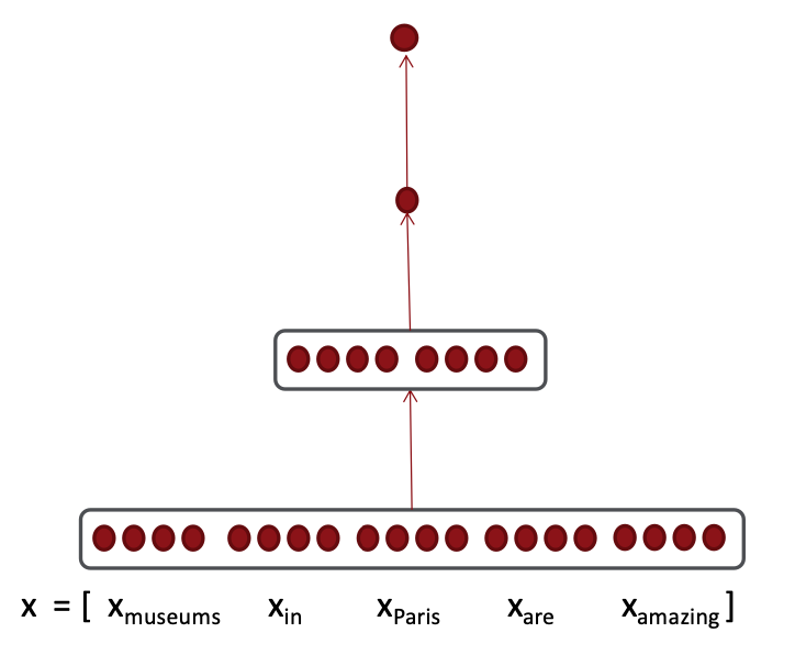
3. Neural Net

$s = u^Th, \ h=f(Wx+b),\ x(input)$

Reference. Stanford CS224n, 2021

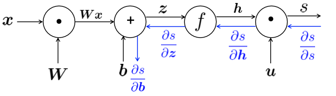
Break up equations into simple pieces: Apply the chain rule, and write out the Jacobians
\[\begin{align} &\dfrac{\partial s}{\partial b} \rightarrow h=f(Wx+b) \rightarrow h = f(z) ,\ z=Wx+b \\ \\ &\dfrac{\partial s}{\partial b} = \dfrac{\partial s}{\partial h}\dfrac{\partial h}{\partial z}\dfrac{\partial z}{\partial b} = u^Tdiag(f'(z))I \end{align}\]
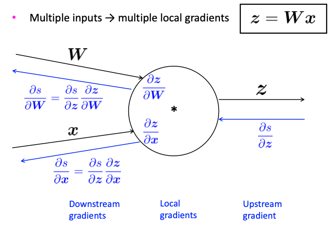
Reusing computation, Find $\dfrac{\partial s}{\partial W}$
\[\begin{align} &\dfrac{\partial s}{\partial W} = \dfrac{\partial s}{\partial h}\dfrac{\partial h}{\partial z}\dfrac{\partial z}{\partial W} \rightarrow \dfrac{\partial s}{\partial h}\dfrac{\partial h}{\partial z} \text{ duplicated computation}\\ \\ &\dfrac{\partial s}{\partial W} = \delta\dfrac{\partial z}{\partial W},\ \dfrac{\partial s}{\partial b} = \delta\dfrac{\partial z}{\partial b} = \delta \\ \\ &\delta = \dfrac{\partial s}{\partial h}\dfrac{\partial h}{\partial z} = u^T \circ f'(z), \delta \text{ is the local error signal} \end{align}\]
Derivative with respect to Matrix

Output Shape $\dfrac{\partial s}{\partial W}$ is $W \in \mathbb{R}^{n \times m}$

Instead we use the shape convention: the shape of the gradient is the shape of the parameters
\[\dfrac{\partial s}{\partial W} = \begin{bmatrix} \dfrac{\partial s}{\partial W_{11}} & \cdots & \dfrac{\partial s}{\partial W_{1m}} \\ \vdots & \ddots & \vdots\\ \dfrac{\partial s}{\partial W_{n1}} & \cdots & \dfrac{\partial s}{\partial W_{nm}} \end{bmatrix}, \text{ n by m}\]
$\delta$ is going to be in our answer, And the other term should be x because z = Wx + b.
\[\dfrac{\partial s}{\partial W} = \delta \dfrac{\partial z}{\partial W} = \delta\dfrac{\partial}{\partial W}(Wx+b)\]
Get a row component derivative by a W,
\[\dfrac{\partial z_i}{\partial W_{ij}}=\dfrac{\partial }{\partial W_{ij}}W_ix +b_i = \dfrac{\partial }{\partial W_{ij}}\textstyle\sum_{k=1}^dW_{ik}x_k = x_j\]
A row component derivative by a W is same as ‘a’ x.

$\delta$ is local error signal at z, x is local input signal,
\[\begin{align} \dfrac{\partial s}{\partial W} &= \delta^T x^T \\ [n \times m] &= [n \times 1][1 \times m] \\ &=\begin{bmatrix} \delta_1\\ \vdots\\ \delta_n\ \end{bmatrix} \begin{bmatrix} x_1, \cdots ,x_m \end{bmatrix} = \begin{bmatrix} \delta_1 x_1 & \cdots &\delta_1 x_m\\ \vdots & \ddots & \vdots \\ \delta_n x_1 & \cdots &\delta_n x_m \end{bmatrix} \end{align}\]
Why the Transpose? Hacky answer: this makes the dimensions work out!

Similarly, $\dfrac{\partial s}{\partial b} = h^T \circ f’(z)$ is a row vector. But shape convention says our gradient should be a column vector because b is a column vector.
1. Use Jacobian form as much as possible, reshape to follow the shape convention at the end. But at the end, transpose $\dfrac{\partial s}{\partial b}$ to make the derivative a column vector, resulting in $\delta^T$
2. Always follow the shape convention. Look at dimensions to figure out when to transpose and/or reorder terms. Or the error message $\delta$ that arrives at a hidden layer has the same dimensionality as that hidden layer

4. Backpropagation

$s = u^Th, \ h=f(Wx+b),\ x(input)$

Reference. Stanford CS224n, 2021

Upstream, Downstream

Reference. Stanford CS224n, 2021
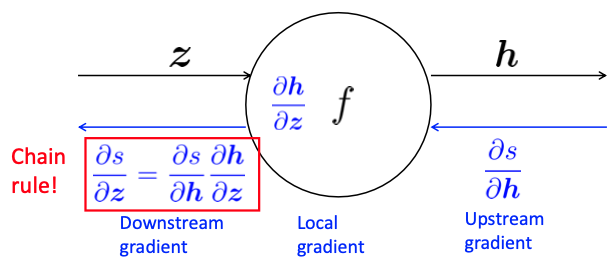
Single Node

Reference. Stanford CS224n, 2021
Example

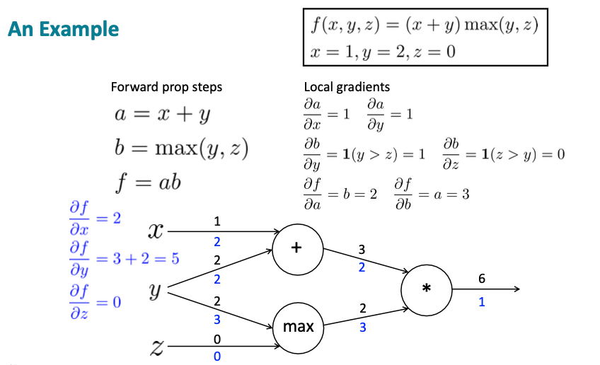
Reference. Stanford CS224n, 2021
Practice: https://github.com/karpathy/micrograd

5. Back-Prop in General Computation

Fprop: visit nodes in topological sort order

Compute value of node given predecessors
Bprop
- initialize output gradient = 1
- visit nodes in reverse order:
  
  Compute gradient wrt each node using gradient wrt successors
  
  ${y1, y2, \cdots, y_n}$ = successors of x
  
  $\dfrac{\partial z}{\partial x} = \displaystyle\sum_{i=1}^{n}\dfrac{\partial z}{\partial y_i}\dfrac{\partial y_i}{\partial x}$

If Done correctly, BIG O() complexity of fprop and Bprop is the same.
In general, our nets have regular layer-structure and so we can use matrices and Jacobians.
Automatice Differentiation
- The gradient computation can be automatically inferred from the symbolic expression of the fprop
- Each node type meeds to know how to compute its output and how to compute the gradient wrt its inputs given the gradient wrt its output
- Modern DL framework(Tensorflow, PyTorch, etc.) do back propagation for you but mainly leave layer/node writer to hand-calculate the local derivative.

Sample Code

Backprop Implementation

  class ComputationalGraph(object):
      #...
      def forward(inputs):
              #1. pass inputs to input gates
              #2. forward the computational graph
              for gate in self.graph.nodes_topologically_sorted():
                  gate.forward()
              return loss # the final gate in the graph outputs the loss
      def backward():
              for gate in reversed(self.graph.nodes_topologically_sorted()):
                  gate.backward()
              return inputs_gradients	

Forward/Backward API

  """
      x
       \
         * ---> z
       /
      y
  """
  class MultiplyGate(object):
      def forward(x, y):
          z = x*y
          self.x = x # must keep these around!
          self.y = y
          return z
      def backward(dz):
          dx = self.y * dz # [dz/dx * dL/dz]
          dy = self.x * dz # [dz/dx * dL/dz]
          return [dx, dy]

6. Exploding and Vanishing gradients

Read here! https://karpathy.medium.com/yes-you-should-understand-backprop-e2f06eab496b
Problem “Leaky abstraction”
Dying ReLUs
Exploding gradients in RNNs
Clipping

PREVIOUSThe Concept of Neural Network and Technique

NEXTCS224N W2. Neural Network and What is the Dependency Parsing