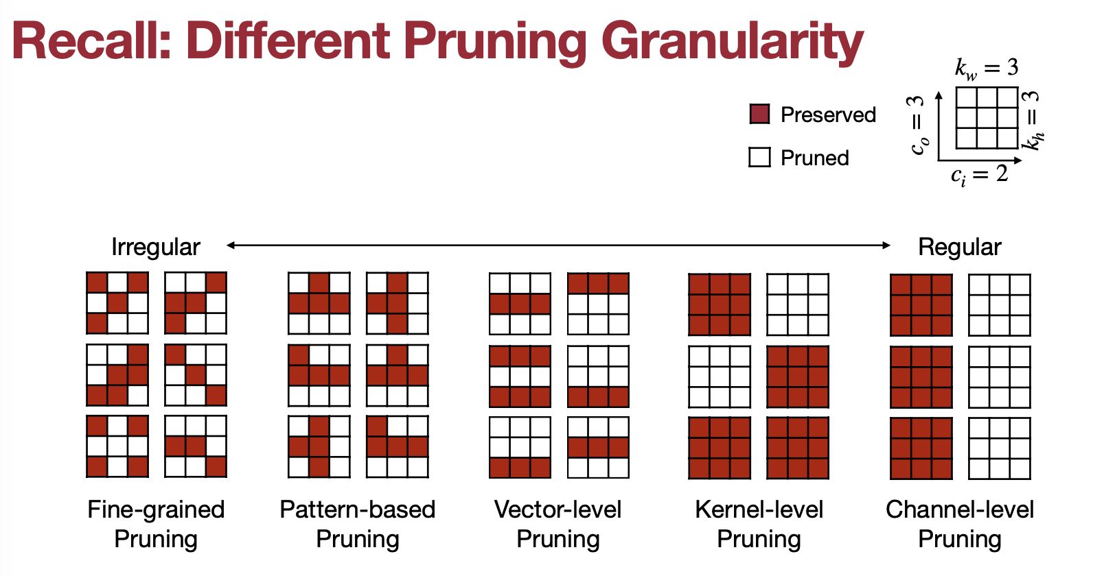
앞서서 MIT에서 Song Han 교수님이 Fall 2022에 한 강의 TinyML and Efficient Deep Learning Computing 6.S965에서 경량화 기법으로는 Pruning을 정리하고 있다. 지난 글에서는 Granularity와 Criterion에 대해서 나눴다면 이번에는 Ratio, Fine-tuning, Lottery Ticket Hypothesis, System Support를 다뤄보고자 한다.
첫 번째 내용으로 Pruning Ratio 부터 시작해보자.
4. Determine the Pruning Ratio
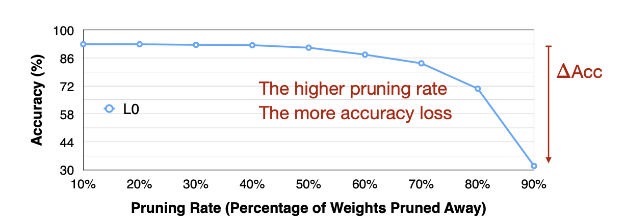
뉴런이나 시냅시의 Pruning을 몇 퍼센트를 해야할까? 강의에서는 각 레이어마다 Senesitivitiy가 다르다 하여, Pruning ratio 또한 달라야 한다고 설명한다. 즉 각각의 레이어마다 Pruning ration을 조정하면서 적정한 값을 찾아야 한다는 것인데, 그 단계를 소개해준다.
- 레이어 $L_i$ 를 고르고 pruning ratio $r \in { 0,\ 0.1, \dots, 0.9}$ 에서 선택한다.
-
Output의 변화치($\Delta ACC_r^i$ )를 각 pruning ratio 마다 측정한다.
Reference. MIT-TinyML-lecture3-Pruning-2 in https://efficientml.ai
-
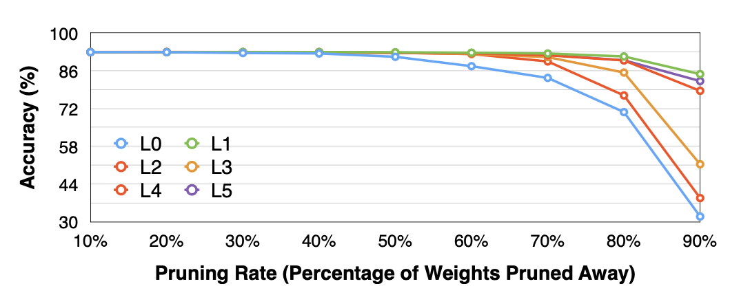
위 과정을 모든 레이어로 반복한다.
Reference. MIT-TinyML-lecture3-Pruning-2 in https://efficientml.ai
-
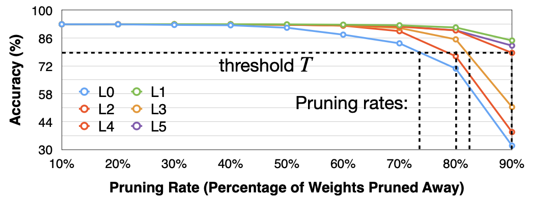
Output(e.g. Accuracty)의 최저점(degradation threshold $T$)를 고른다.
Reference. MIT-TinyML-lecture3-Pruning-2 in https://efficientml.ai
위 과정을 Heuristic으로 진행하지만, 아직 “레이어간 영향”에 대해서는 분석하지 못한다. 그리고 각 레이어마다 Pruning에 따른 Sensitivity 다른데, 근데 레이어마다 파라미터 상태가 같은가? 아니다. 어떤 레이어는 파라미터가 billion에 육박할 수 있고 어떤 레이어는 적은 레이어라 Pruning을 해도 크게 차이가 안날 수 있다. 그럼 모델 전체를 어떻게 Pruning Ratio를 정해야할까?
*참고로 강의에서 최근 모델들은 llama, transfomer과 같은 모델들은 Layer간 동질성을 가지고 있다(반면 CNN은 아니라고 언급한다).
4.0 TL;DR Automatic Pruning
- AutoML for Model Compression: Features + Reinforce Learning → Find out State!
- NetAdapt: To obtain specific objective measure(e.g. latency) with a layer, and iteratively prune layers.
4.1 AutoML for Model Compression
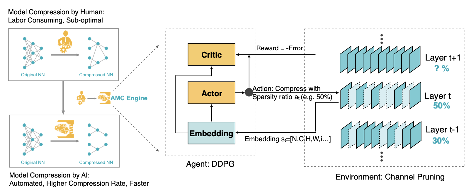
그래서 이야기하는 것이 Song Han교수님 연구실에서 냈던 페이퍼 중 하나인 AutoML이다. AutoML에서는 강화학습 컨셉을 함께 가져온다. DDPG를 이용해서 Reward에 $log(FLOP)$만큼 더 곱해주는 방식을 취한다. 그럼 왜 log(FLOP)일까? 아래 그림을 보면 computation수와 accuracy에 대한 관계가 대략적으로 log function을 취하는 것을 볼 수 있고 이를 이용한 것이라 설명한다.

Reference. AMC: AutoML for Model Compression and Acceleration on Mobile Devices [He et al., ECCV 2018]
*Actor $\pi_{\theta}(a\lvert s)$, Critic $Q^{\pi}_{\theta}(s,a)$
그럼 actor는 어떤 action을 할까? 바로 Sparsity ratio를 조절한다. 그러면 Layer마다 N(Batch size), C(Channel number), H(Height), W(Width), i(index) 와 같은 파라미터를 Embedding를 Decision을 하는 곳에 전달한다 (Latency는 왜 안쓰냐는 학생의 질문이 있었는데, 연구에서는 FLOP이 더 좋은 퍼포먼스를 보였다고 한다. 참고로 Reward는 1 game이 지나고 나서 나온다고 설명한다). 자세한 내용은 추후에 논문을 리뷰하면서 설명하도록 하겠다.
Reference. AMC: AutoML for Model Compression and Acceleration on Mobile Devices [He et al., ECCV 2018]
- Reward → $-Error * log(FLOP)$
- AMC uses the following setups for the reinforcement learning problem
- State: 11 features including layer indices, channel numbers, kernel sizes, FLOPs
- Action: A continuous umber (pruning ratio) $a \in [0, 1)$
- Agent: DDPG agent, since it supports continuous action output
- Reward:
- It can also optimize latency constraints with a pre-built lookup table
- Reference. https://arxiv.org/pdf/1802.03494.pdf
- Code. https://github.com/mit-han-lab/amc.git
결과를 보면 논문에서 결과는 사람이 한 Pruning보다 더 많이 경량화를 한 것을 확인 할 수 있고 아래의 결과에서는 stage를 거치면서 레이어마다 더 공격적으로 Pruning을 진행한 부분을 확인할 수 있다(1x1 convolution vs 3x3 convolution). 참고로 이 연구는 channel pruning 패턴을 이용했다.
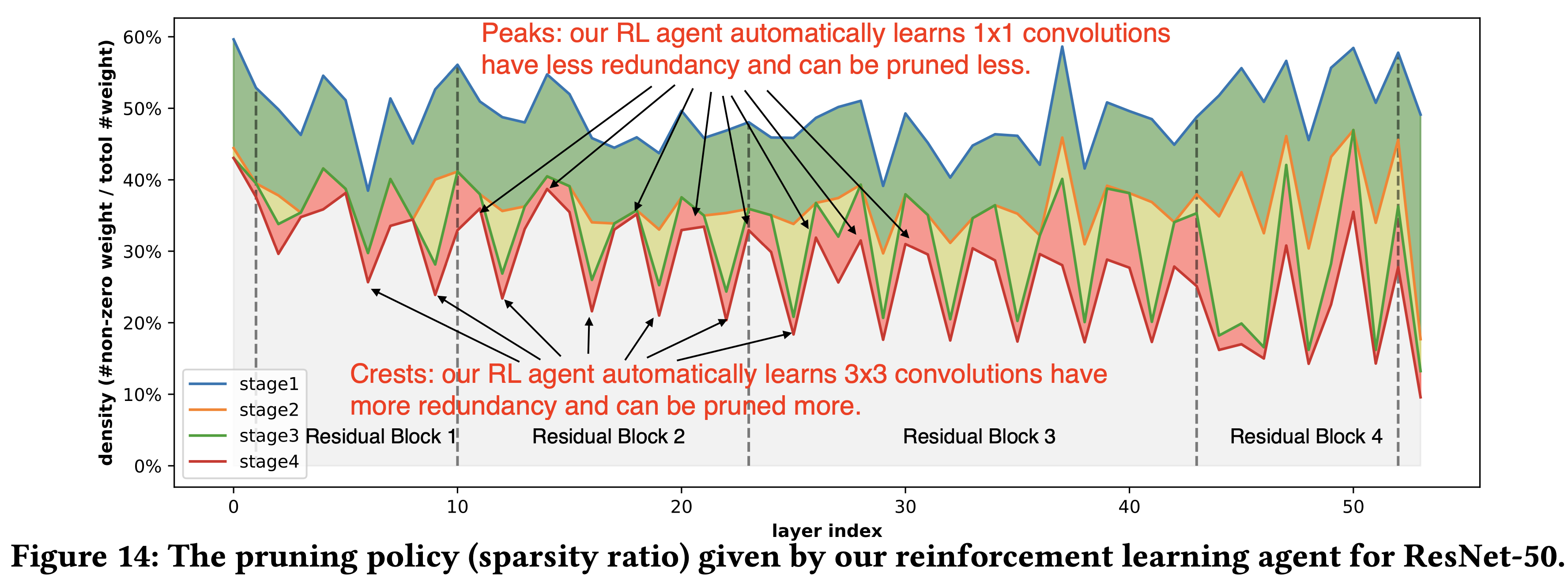
Reference. AMC: AutoML for Model Compression and Acceleration on Mobile Devices [He et al., ECCV 2018]
그리고 이를 Snapdragon이 있는 Galaxy S7 Edge 에서 확인했을 때도 Uniform-shrink 75%를 한 MobileNet보다 Accuracy의 저하를 줄이면서 Latency를 확보하는 것을 표에서도 확인할 수 있다.
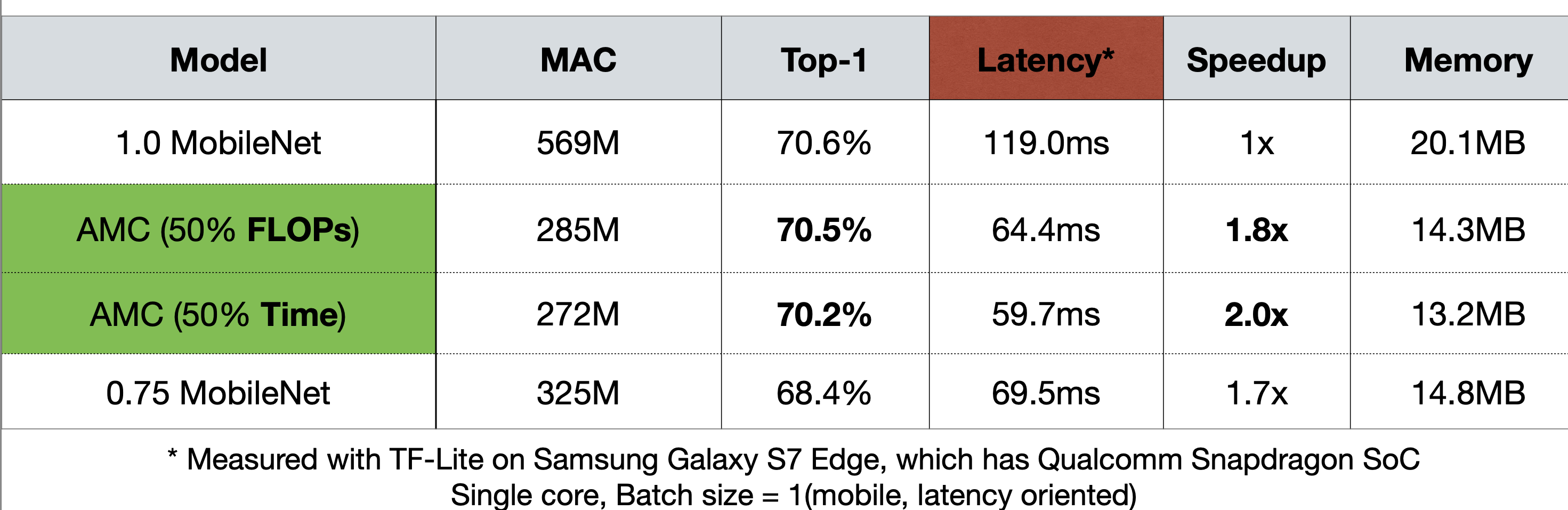
Reference. AMC: AutoML for Model Compression and Acceleration on Mobile Devices [He et al., ECCV 2018]
근데 Uniform-shrink에서 보면 25% 만큼 파라미터를 줄이면서 Latency를 1.7x 만큼 빨라지는 것을 볼 수 있는데, Channel이 25%만큼 줄어들었다고 하면 Latency도 1.25x 만큼 빨라져야 하지 않을까? Convolution 레이어를 생각해보면 된다. Width x Heigh x kernel size x input channel x output channel이 되는데, 여기서 channel 이 N배만큼 준다고 생각하면 전체 연산수(전체 연산수에 비례하게 Latency와 줄어든다고 가정하면)는 quadratic( $N^2$ )만큼 줄게 된다. 그래서 모델의 파라미터가 준 비율보다 더 많이 Latency가 줄어드는 것이다.
4.2 NetAdapt
두번째로 소개하는 논문은 NetAdapt이다. 컨셉이 많이 간단한데, 우선 성능하락폭의 제한선을 먼저 정해두고 그에 만족한다는 전제하에 모델의 각 레이어를 Pruning한다. 그 때 가장 성능이 좋은 경우를 적용하고, 이 과정을 계속 반복한다. 그리고 마지막에 Fine-tune을 넣어서 최종 모델을 얻는다는 내용이다.
- Reference. https://arxiv.org/pdf/1804.03230.pdf
- Code. https://github.com/denru01/netadapt
- A rule-based iterative/progressive method
-
The goal of NetAdapt is to find a per-layer pruning ratio to meet global resource constraint(e.g. latency, energy)

Reference. NetAdapt: Platform-Aware Neural Network Adaptation for Mobile Applications [Yang et al., ECCV 2018]
- For each iteration, it aims to reduce the latency by a certain amount $\Delta R$ (manually defined)
- For each layer $L_k$(k in A-Z in the figure)
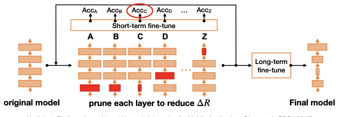
Reference. NetAdapt: Platform-Aware Neural Network Adaptation for Mobile Applications [Yang et al., ECCV 2018]
- Prune the layer s.t. the latency reduction meets $\Delta R$ (based on a pre-built lookup table)
- Short-term fine-tune model (10k iterations); measure accuracy after fine-tuning
- Repeat until the total latency reduction satisfies the constraint
- Long-term fine-tune to recover accuracy
여기까지 Pruning ratio를 정하는 방법을 두 가지 논문에서 살펴봤다. 이렇게 Pruning을 하고 나면, 그 다음에 하는 단계로 소개하는 것은 Fine-tuning이다.
5. Fine-tune/Train Pruned Neural Network
우선 Learning rate는 보통 1/100 혹은 1/10배로 원래 Learning rate보다 작게 설정한다고 한다.
- How do we fine-tune neural-network pruning?
- After pruning, the model may decrease, especially for larger pruning ratio.
- Fine-tuning the pruned neural networks will help recover the accuracy and push the pruning ratio higher
- Learning rate for fine-tuning is usually 1/100 or 1/10 of the original learning rate
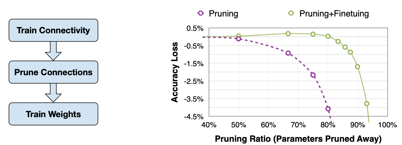
Learning Both Weights and Connections for Efficient Neural Network [Han et al., NeurIPS 2015]
그리고 0부터 100%처럼 크게 Pruning을 하고나서 바로 Fine-Tuning을 하는 방법도 있지만, 20%씩 작은 스텝으로 Pruning을 하고 Fine-tuning을 그 다음에 하면서 반복적으로 Pruning-Fine tuning을 하는 방법도 Iterative Pruning이라고 소개한다.
5.1 Iterative Pruning

Learning Both Weights and Connections for Efficient Neural Network [Han et al., NeurIPS 2015]
- Consider pruning followed by a fine-tuning is one iteration.
- Iterative pruning gradually increases the target sparsity in each iteration
- Boost pruning ratio from 5X to 9X on AlexNet compared to single-step aggressive pruning.
결과는 위에서 보이다 시피, Iterative 의 경우가 더 성능하락폭을 줄일 수 있는 것을 볼 수 있다. 하지만 Iterative는 engineering관점에서는 더 시간이 든다!
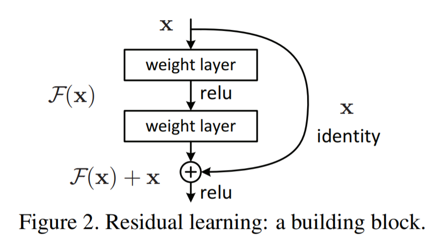
여기서 교수님이 by-pass layer(Skip Connection?)에 대해서 언급한다. by-pass의 경우 이전, 이후 레이어에 dependent하기 때문에 Pruning ratio를 정하는데 더 까다롭다고 한다.
Learning Both Weights and Connections for Efficient Neural Network [Han et al., NeurIPS 2015]
5.2 Regularization
Fine-tuning을 하면서 하나 더 소개하는 것은 모델 훈련에서도 쓰이는 Regularization이다. 간단하게 식을 짚고 넘어가도록 하자.
-
This regularization penalize non-zero parameters and encourage smaller parameter.
-
L1-Regularization: $L’ = L(x;W) + \lambda\lvert W \lvert$
-
L2-Regularization: $L’ = L(x;W) + \lambda\lvert\lvert W \lvert\lvert^2$
-
Example Papers:
- Magnitude-based Fine-grained Pruning applies L2 regularization on weights
- Network Slimming applies smooth-L1 regularization on channel scaling factors.
- Learning Efficient Convolutional Networks through Network Slimming [Liu et al., ICCV 2017]
- Learning Both Weights and Connections for Efficient Neural Network [Han et al., NeurIPS 2015]
6. Lottery Ticket Hypothesis
스터디 초반에도 나온 질문이 하나 있다. “Scratch에서부터 그냥 Pruning을 해서 모델을 만들면 안되나요?” 그리고 Pruning은 마치 Dropout과도 비슷하게 생각될 수도 있다. 아, 물론 Dropout은 목적이 overfitting 방지로 다르고, Random하게 수가 다른 파라미터를 줄이는 것으로 Pruning은 Inference 속도를 올릴 수 있다는 측면에서 다르다. Pruning에서 파라미터를 줄인다는 것은 LLM과 같은 거대 파라미터를 가진 모델에서 “over-parameterization과 redundancy”는 local minimum을 구하는 과정이나 non-convex 문제를 푸는 포인트와 연관지어서도 생각해 볼 수 있다.
다시 요점으로 돌아가 보자. 그럼 Sparsity를 찾을 수 있을까? 이에 대해서 Lottery Ticket Hypothesis 논문이 비교적 간단한 문제(CIFAR10, MNIST)를 푸는 모델에 대해서 이야기하는 부분이 바로 이번 파트이다(ImageNet은 Challenging하다). 결과부터보자면, 무작위로 Sparse Network를 고른 경우는 Accuracy가 다시 돌아오지 못하지만, Training을 통해 Sparse Mask를 정한 후에 초기 단계부터 시작한 Sparse Network의 경우는 Accuracy를 어느정도 보존하는 것을 볼 수 있다.
- Can we train a sparse neural network from scratch?
-
Contemporary experience tells us the architectures uncovered by pruning are harder to train from the start reaching low accuracy than the original networks.

The Lottery Ticket Hypothesis: Finding Sparse, Trainable Neural Networks [Frankle et al., ICLR 2019]
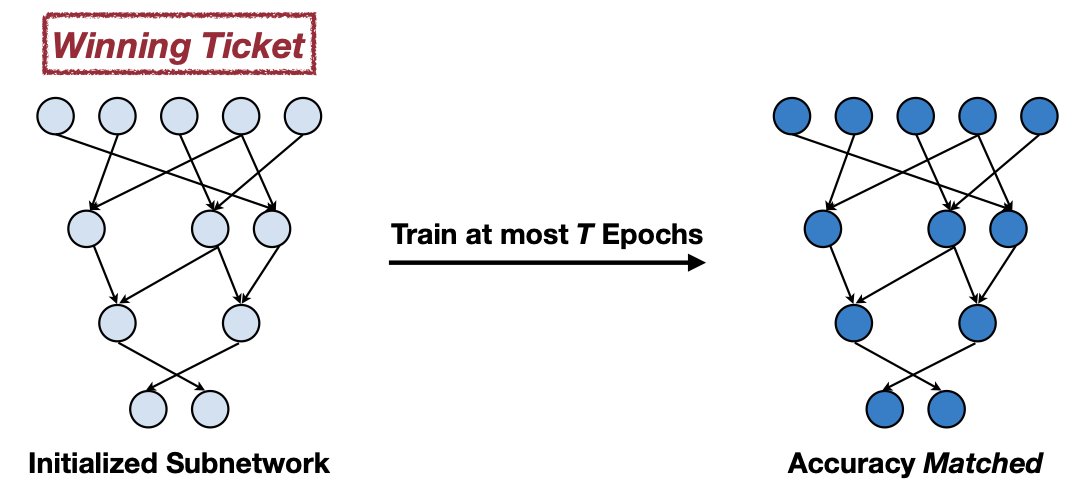
- The Lottery Ticket Hypothesis: A randomly-initialized, dense neural network contains a subnetwork that is initialized such that — when trained in isolation — it can match the test accuracy of the original network after training for at most the same number of iterations.
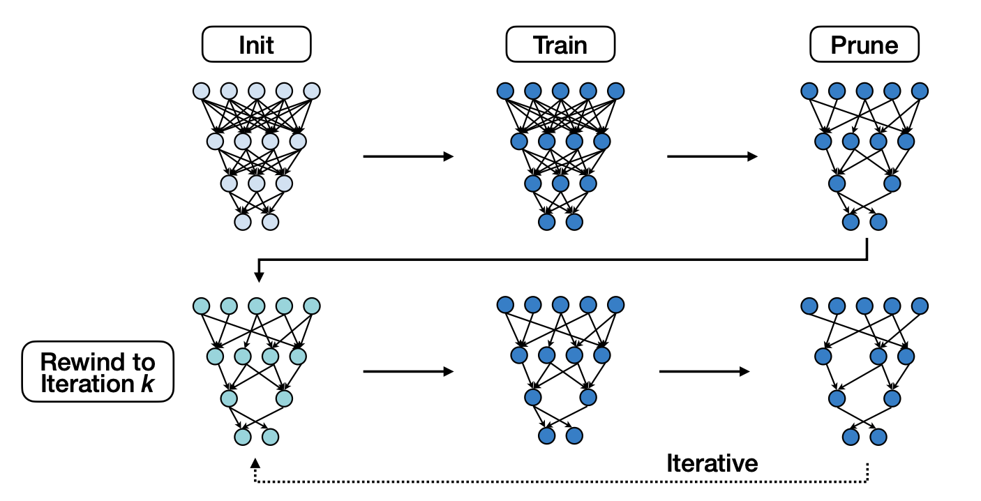
6.1 Iterative Magnitude Pruning
방식은 간단하다. Training통해 Pruning mask를 우선 구한 후 정해진 Sparse Network를 이전 Training횟수와 동일하게 Iterative로 Magnitude를 기준으로 훈련시킨다.
-
If training is isolation in sub-network, it can match the test accuracy after training for at most the same number of iterations.
MIT-TinyML-lecture03-Pruning-2 in https://efficientml.ai
6.2 Scaling Limitation: The Lottery Ticket Hypothesis with Rewinding
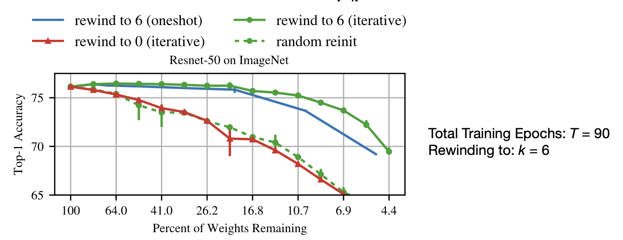
결과는 처음에 말한 것과 동일하다. training을 하지 않은 상태에서 Sparse Network를 고른 경우는 Accuracy가 Sparsity가 커질수록 떨어지는 것을 볼 수 있다. 반면 training을 한 상태에서 Sparse Network를 고른 경우 1번에 training 횟수만큼 훈련을 시키던, iterative하게 훈련을 시키던 Accuracy가 어느정도 유지되는 것을 볼 수 있다. 하지만, 이는 분명 간단한 테스크에 Deep하지 않은 Network의 경우이다.
- TL;DR intital value is not iteration $t=0$, but $t=k$
- Resetting the weights to the very initial value $W_{t=0}$ works for small-scale tasks such as MNIST(32x32) and CIFAR-10(32x32), and fails on deep networks.
-
Instead, it is possible to robustly obtain pruned subnetworks by resetting the weights to the values after a small number of k training iterations, that is $W_{t=k}$
MIT-TinyML-lecture03-Pruning-2 in https://efficientml.ai
-
The Lottery Ticket Hypothesis with Rewinding:
Consider a dense, randomly-initialized neural network $f(x;W_0)$ that trains to accuracy $a^{\ast}$ in $T^{\ast}$ iterations. Let $W_t$ be the weights at iteration $t$ of training. There exist an iteration $k « T^{\ast}$ and fixed pruning mask $m \in {0, 1}^{\lvert W \lvert}$ (where $\lvert\lvert m \lvert\lvert_1 « \lvert W \lvert$) such that subnetwork $m \odot W_k$ trains to accuracy $a \geq a^{\ast}\ in\ T \leq T^{\ast}-k$ iterations.
MIT-TinyML-lecture03-Pruning-2 in https://efficientml.ai
7. System Support for Sparsity
마지막 파트는 하드웨어적으로 Sparsity를 지원하는 경우를 살펴볼 것이다. 결과로는 당연히 FLOP의 감소를 볼 수 있을 것이다.
MIT-TinyML-lecture03-Pruning-2 in https://efficientml.ai
쉽게 쓸 수 있는 방법은 Channel-level pruning이다. 아래에 레이어 파라미터를 바꾸면서 Pruning이 가능하다.
-
Channel-level Pruning → No need for specialized system support

MIT-TinyML-lecture03-Pruning-2 in https://efficientml.ai
외에 Efficient Inference Engine(EIE), Load Balance Aware Pruning, Fine-grained Pruning 패턴에서 SpMM, CSR Format, GPU Support for SpMM, Load balancing, Pattern-based Pruning에서는 Vector-level, Kernel-level Pruning, Filter Kernel Reorder, Filter Kernel Weight(FKW) Format, Load Redundancy Elimination(LRE) by GPU Support, 마지막으로 TorchSparse & PointAcc까지 살펴볼 것이다. 여러 논문들이지만, 핵심은 어떻게 파라미터를 잘 분포시키는가와 인덱스를 어떤 방식으로 나타낼 것인가를 생각하면서 따라오면 되겠다.
7.1 EIE: Efficient Inference Engine
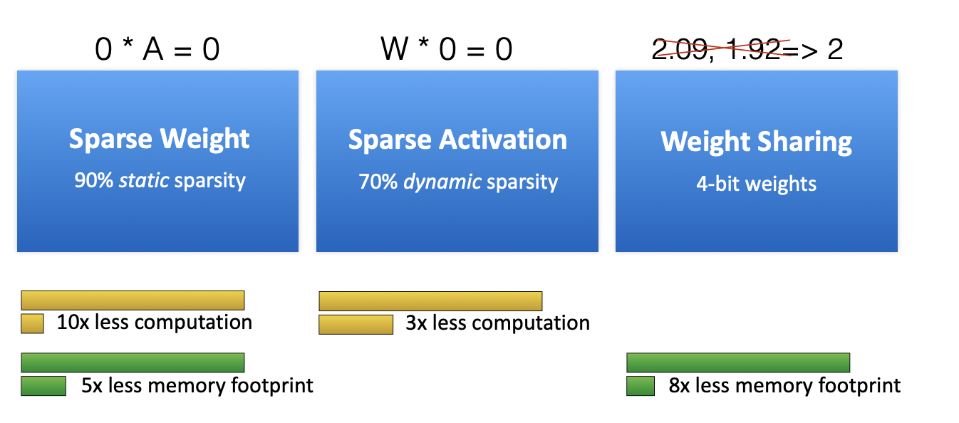
아래 그림에서 보면 90% Sparse weight로 10배의 computation이 줄어든 것을 볼 수 있다. 반면 메모리는 5배만큼만 줄어드는데, 왜 Weight와 동일하지 않을까? 바로 인덱스 때문이다. 그리고 Activation 경우에는 Dynamic한 특징 때문에 Weight만큼 줄일 수는 없는 것도 볼 수 있다.
-
The first DNN Accelerator for Sparse and Compressed Model
EIE: Efficient Inference Engine on Compressed Deep Neural Network [Han *et al.,* ISCA 2016]
-
Parallelization on Sparsity considering locally and physically memory allocation by designing ASIC
그럼 이제 어떻게 인덱스를 둘지 알아보자. EIE에서는 PE(multiple processing elements) 라는 하나의 계산 유닛이 Weight 의 특정 행을 맡는다. 예를 들어 아래의 경우, 연산은 $b_i = ReLU\huge( \large \sum_{j=0}^{n-1} W_{ij}a_j \huge{)}$ 이고 $w_{0,0}, w_{0,1},0, w_{0,3}, 0, 0, w_{4,2}, w_{4,3}$를 $PE0$ 가 맡는다.
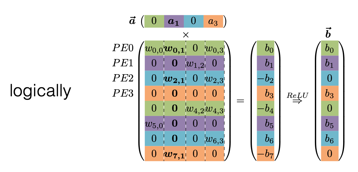
EIE: Efficient Inference Engine on Compressed Deep Neural Network [Han *et al.,* ISCA 2016]
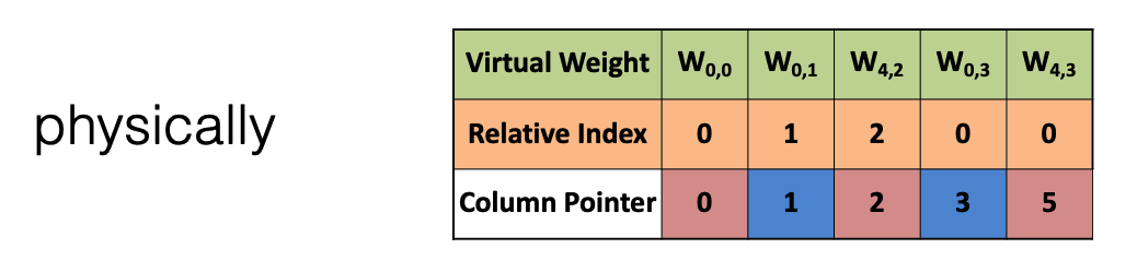
그럼 $PE0$ 는 이 파라미터들을 아래의 인덱스 형태로 기억한다. 이는 compressed sparse column(CSC)이라는 형태를 사용한다. 잠깐 설명하자면, 아래의 표처럼 각 Weight를 Relative Index와 Column Pointer로 표기한다. Relative Index은 weight를 차례로 인덱싱할 때, 0인 경우는 저장하지 않으므로 그 때문에 건너 뛴 weight의 수를 나타낸다. 예를 들어 $W_{0,1}$ 과 $W_{4,2}$ 사이에 0이 두개이므로 $W_{4,2}$의 Relative Index는 2가 된다.
*Column Pointer는 아직 이해가 가지 않는 부분이 CSC format은 이름 그대로 Weight의 Column을 나타내지만 여기서 다른 Weight와 달리 $W_{4,3}$에서 5라고 표기돼 앞선 Column 설명이 맞지 않다(논문에서도 찾을 수 없어 혹시 아는 부분이 있다면 댓글 부탁드려요 !).
EIE: Efficient Inference Engine on Compressed Deep Neural Network [Han *et al.,* ISCA 2016]
이를 하드웨어 로직으로 표현한 것이 아래와 같다. 이 논문에서의 핵심은 Act Queue, 그리고 Weight Decoder와 Address Accum(Index)이 되겠다. Encoding된 sparse weight matrix W에 Compressed Sparse Column (CSC) format이 적용된 것이다. 여기서 Act Queue가 Multi PE를 이용해서 Load Balance 역할을 하고, Act Index를 통해서 Activation Sparsity 역할을 맡는다. 그리고 앞서서 설명한 Weight Decoder와 Address Accum(Index)는 Weight Sparsity를 맡는다.
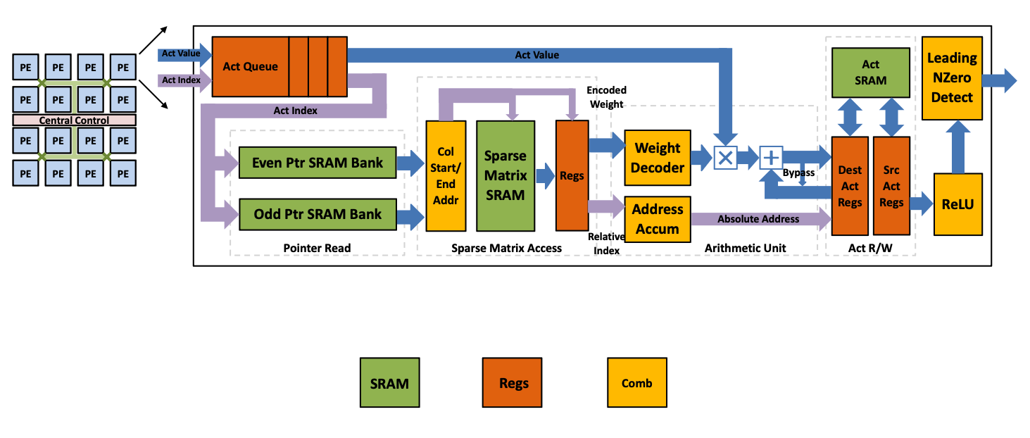
EIE: Efficient Inference Engine on Compressed Deep Neural Network [Han *et al.,* ISCA 2016]
이 결과는 논문을 보면 16bit Int 까는 성능하락폭이 1%미만이다. FLOP Reduction, 에너지 효율성 등등이야 말할 것도 없으니 논문을 참고하자.
The first principle of efficient AI computing is to be lazy: avoid redundant computation, quickly reject the work, or delay the work.
- Generative AI: spatial sparsity [SIGE, NeurlPS’22]
- Transformer: token sparsity, progressive quantization [SpAtten, HPCA’21]
- Video: temporal sparsity [TSM, ICCV’19]
- Point cloud: spatial sparsity [TorchSparse, MLSys’22 & PointAcc, Micro’22]
We envision future AI models will be sparse at various granularity and structures. Co-designed with specialized accelerators, sparse models will become more efficient and accessible.
EIE를 통해 이야기하고 싶었던 부분은 경량화에서 불필요한 연산을 최대한 피하고 한 번에 그 연산을 처리하도록 하는 것이었다.
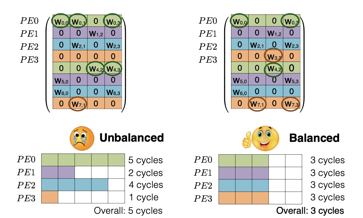
7.2 Load Balance Aware Pruning
두 번째 방식은은 앞선 EIE에서 Pruning시에 Load Balacne를 고려했다고 한다. 말인 즉슨, PE마다 가지는 Weight의 수를 동일하게 했다는 내용이다. 방향만 알아두고 자세한 내용이 궁금하다면 페이퍼로!
ESE: Efficient Speech Recognition Engine with Sparse LSTM on FPGA [Han et al., FPGA 2017]
- Sweet spot: Same Accuracy, Better Speed up
7.3 Fine-grained Pruning
세번째부터는 Fine-grained한 Pruning 패턴에서 방법을 알아보자
MIT-TinyML-lecture03-Pruning-2 in https://efficientml.ai
-
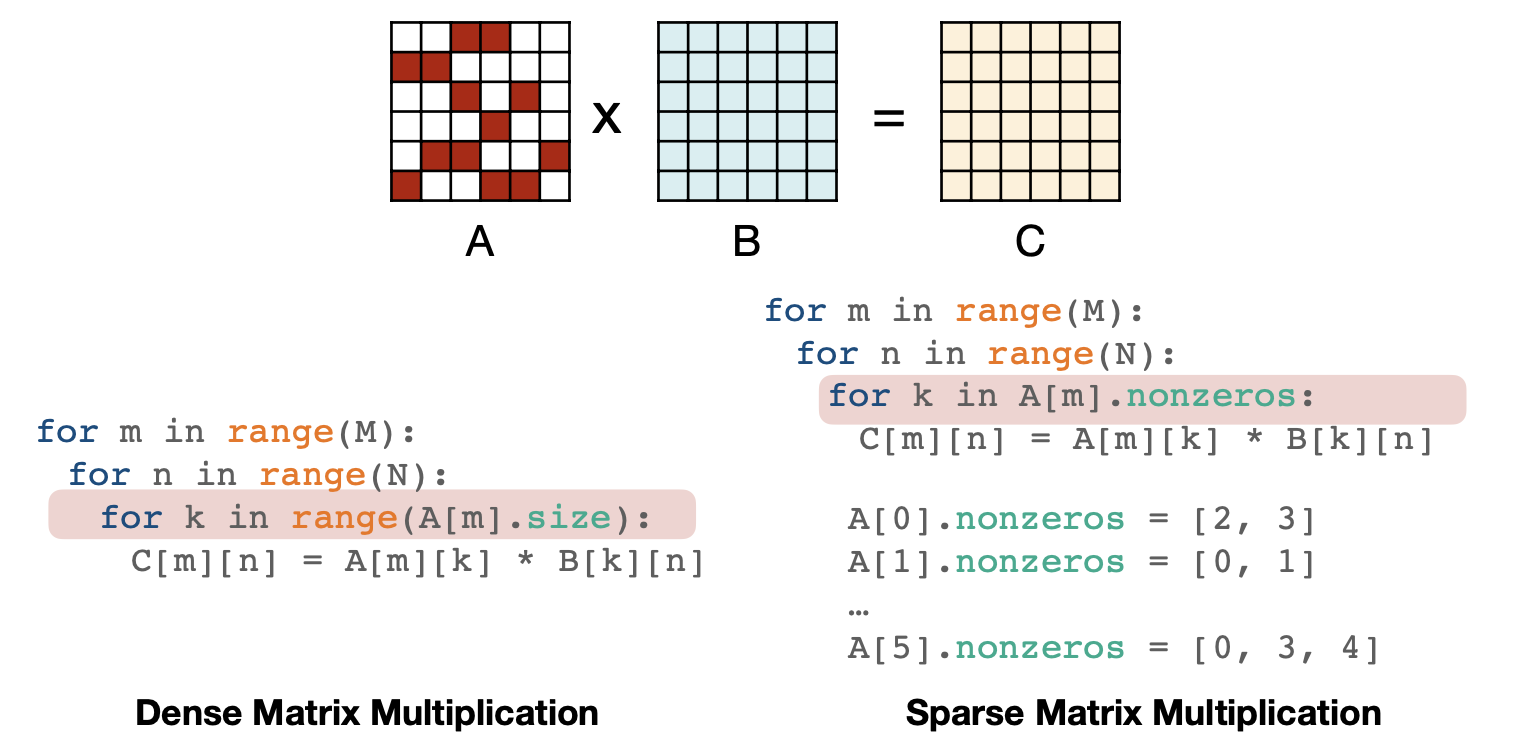
Sparse Matrix-Matrix Multiplication(SpMM)
첫 번째는 Sparse Matrix-Matrix Multiplication으로 non-zero인 경우의 index를 저장해놓는 방식이다.
ESE: Efficient Speech Recognition Engine with Sparse LSTM on FPGA [Han et al., FPGA 2017]
-
CSR Format for Sparse Matrices
두 번째는 SpMM으로 표현한 파라미터를 CSR Format으로, 행과 열, 그리고 그에 맞는 파라미터를 각각 벡터의 형태로 저장한다.
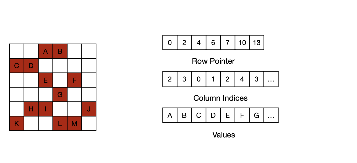
MIT-TinyML-lecture03-Pruning-2 in https://efficientml.ai

MIT-TinyML-lecture03-Pruning-2 in https://efficientml.ai
-
GPU Support for SpMM
마지막은 이렇게 표현한 SpMM을 지원하는 GPU에 대한 내용이다. cuSPARSE 라이브러리가 이런 기능을 제공하는데, cuBIAS와 비교해서 Sparsity에 따른 Runtime이 더 빠른 것을 볼 수 있다.

Sparse GPU Kernels for Deep Learning [Gale et al., SC 2020]
그럼 어떻게 동작할까? 행과 열로 추린 Weight Matrix에서 이들을 모은 다음 다시 작은 단위로 쪼개 Thread에 분배하는 방식이다. 자세한 방식은 코드를 참고하자.
MIT-TinyML-lecture03-Pruning-2 in https://efficientml.ai
// Reference. MIT-TinyML-lecture03-Pruning-2 in [https://efficientml.ai](https://efficientml.ai/) 1 template <int kBlockItemsK, int kBlockItemsX> 2 __global__ void SpmmKernel( 3 SparseMatrix a, Matrix b, Matrix c) { 4 // Calculate tile indices. 5 int m_idx = blockIdx.y; 6 int n_idx = blockIdx.x * kBlockItemsX; 7 8 // Calculate the row offset and the number 9 // of nonzeros in this thread block's row. 10 int m_off = a.row_offsets[m_idx]; 11 int nnz = a.row_offsets[m_idx+1] - m_off; 12 13 // Main loop. 14 Tile1D c_tile(/*init_to=*/0); 15 for(; nnz > 0; nnz -= kBlockItemsK) { 16 Tile1D a_tile = LoadTile(a); 17 Tile2D a_tile = LoadTile(a); 18 c_tile += a_tile * b_tile; 19 } 20 21 // Write 22 StoreTile(c_tile, c); 23 } -
Load balancing
이 과정에서 한 가지 더 고려하는 것은 Load Balancing 이다. 컨셉은 이전에 설명했으니 자세한 내용은 논문을 참고!
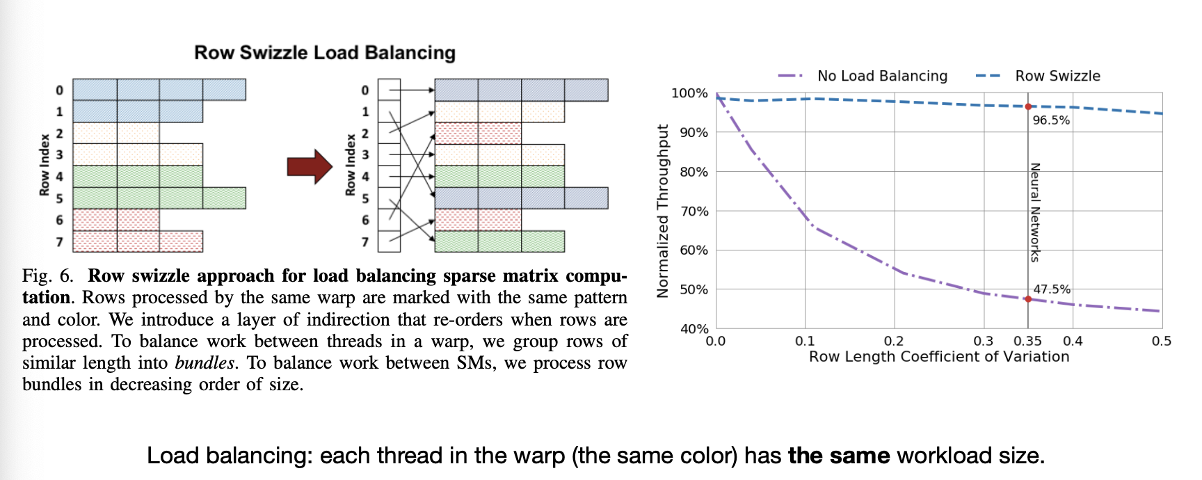
MIT-TinyML-lecture03-Pruning-2 in https://efficientml.ai
7.4 Pattern-based, Vector-level, Kernel-level Pruning
이번엔 Pattern-based Pruning 패턴이다.
- Reference. Block Sparse Format [NVIDIA, 2021]
-
Block Sparse Matrix-Matrix Multiplication(SpMM)

MIT-TinyML-lecture03-Pruning-2 in https://efficientml.ai
Fine-Grained와 다른 점은 index외에 “Block 별 index”가 추가 됐다는 점이다.
-
Block-Ellpack Format: “Remember Block Location”

MIT-TinyML-lecture03-Pruning-2 in https://efficientml.ai
-
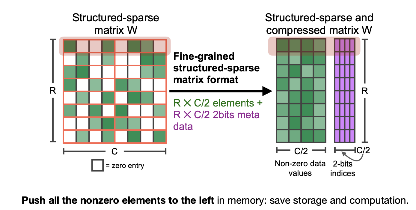
M:N Sparsity
M:N Sparsity에서는 Block별로 따로 고려하진 않고, 행별로 non-zero 파라미터를 모으고 그에 대한 index를 기억한다.
- Accelerating Sparse Deep Neural Networks [Mishra et al., arXiv 2021]
-
Non-zero data value + 2bit metadata
MIT-TinyML-lecture03-Pruning-2 in https://efficientml.ai
그럼 Multiplex 하드웨어 유닛으로 이를 구현할 수 있다.
- System Support for M:N Sparsity
-
Tensor core 는 Sparse를 FP16부터 지원한다!

MIT-TinyML-lecture03-Pruning-2 in https://efficientml.ai
[Q] M:N Sparsitiy를 마무리 짓기 전에 NVIDIA A100에서 Dense, Sparse 네트워트를 비교하는 결과표를 보여준다. 이 표를 보면서 Sparse로 넘어가면서 Speed 적인 성능이 Accuracy의 하락이 거의 없는 상태로 올라간다고 이야기한다. 하지만 궁금한 점은 과연 73-84%의 Accuracy를 가진 네트워크가 사용할 가치가 있을까? 그리고 만약 Accuracy가 더 높아진다면 Sparse는 어떻게 네트워크에 영향을 미칠지가, 그리고 다른 Task에서는 어떻게 영향을 줄지가 궁금해진다.
[A] 논문을 살펴보면 Accuracy에 초점을 맞추기 보단 성능 하락폭에 초점을 맞춘다. 이후에 LLM과 같은 사이즈가 큰 모델의 경우에는 어떻게 결과가 나올지 궁금하다.
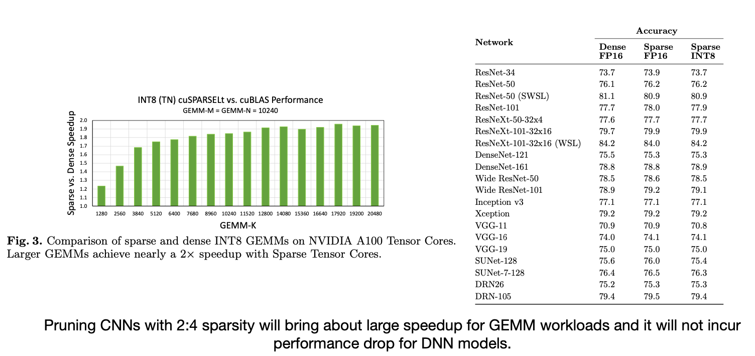
Accelerating Sparse Deep Neural Networks [Mishra et al., arXiv 2021]
7.5 Pattern-Based Pruning: GPU Support
그럼 GPU Support는 내부적으로 어떻게 동작할까?
Accelerating Sparse Deep Neural Networks [Mishra et al., arXiv 2021]
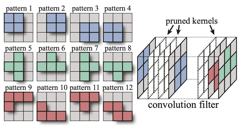
- Reference. An Efficient End-to-End Deep Learning Training Framework via Fine-Grained Pattern-Based Pruning [Zhang et al., arXiv 2020]
- For each output channel in the convolution filter, either prune it away or select its sparsity pattern from a predefined set. → How do model get “sparsity pattern“?
- Problem: Load imbalance between different channel groups (different number of pruned kernels)
논문에서는 “파라미터의 분포가 채널간 그룹에서 균등하게 분포되지 못함”을 집는다. 그리고 그에 대한 해결 방법을 3가지 순서로 차례로 기술한다.
-
Method 1. Filter Kernel Reorder
첫번째는 Kernel을 재배열하는 것이다. 행을 기준으로 Non-zero Weight의 수가 동일한 행끼리 Group을 지어 재배치한 후, 0번째 index부터 빈 곳이 없도록 채워 담는다.
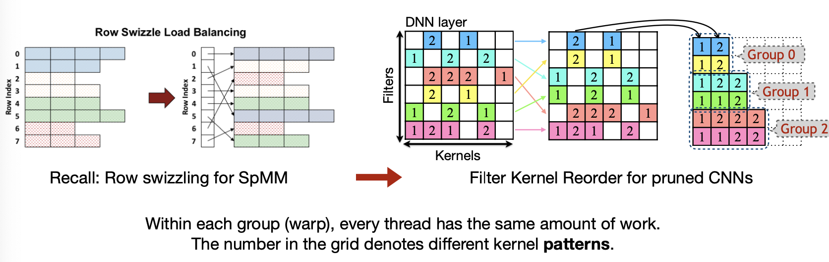
Sparse GPU Kernels for Deep Learning [Gale et al., SC 2020], PatDNN: Achieving Real-Time DNN Execution on Mobile Devices with Pattern-based Weight Pruning [Niu et al., ASPLOS 2020]
-
Method 2. Filter Kernel Weight(FKW) Format
두 번째는 이렇게 재 배열한 파라미터를 아래와 같이 index로 기억한다.
- Offset array: N개의 파라미터가 있다면 각 행에 시작하는 index
- Reorder array: 재배열전 기존에 행의 index
- Index array: 각 파라미터의 행에서의 기존에 index
- Stride array: 필터수의 증가량
- Weight array: 각 커널마다 weight를 vector의 형태로 저장
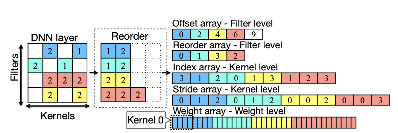
PatDNN: Achieving Real-Time DNN Execution on Mobile Devices with Pattern-based Weight Pruning [Niu et al., ASPLOS 2020]
- It wants to order weight as a sequence!
-
Method 3. Load Redundancy Elimination(LRE)
세번째는 불필요하게 메모리를 불러오는 것을 줄이는 방식이다. 아래 그림에서 보면 Kernel과 Filter에 대해서 Input Feature와 계산시 각각 공통되는 부분을 한 번만 메모리로 불러와 계산할 수 있음을 보여준다.
PatDNN: Achieving Real-Time DNN Execution on Mobile Devices with Pattern-based Weight Pruning [Niu et al., ASPLOS 2020]
PatDNN: Achieving Real-Time DNN Execution on Mobile Devices with Pattern-based Weight Pruning [Niu et al., ASPLOS 2020]
7.6 TorchSparse & PointAcc: Activation Sparsity for Sparse Convolution
마지막은 2023년강의에서 소개하는 TorchSparce와 PointAcc 논문에서 나오는 Activation Sparsity 방식이다. 이 두 논문은 PointCloud에서 Pruning을 소개해주는데 하나씩 살펴보자.
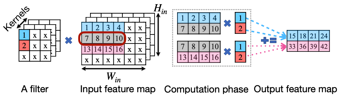
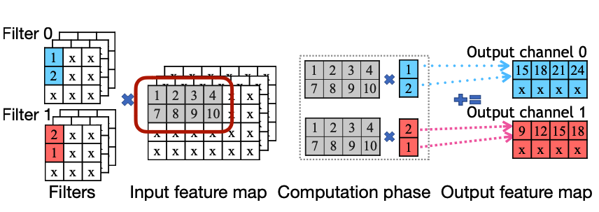
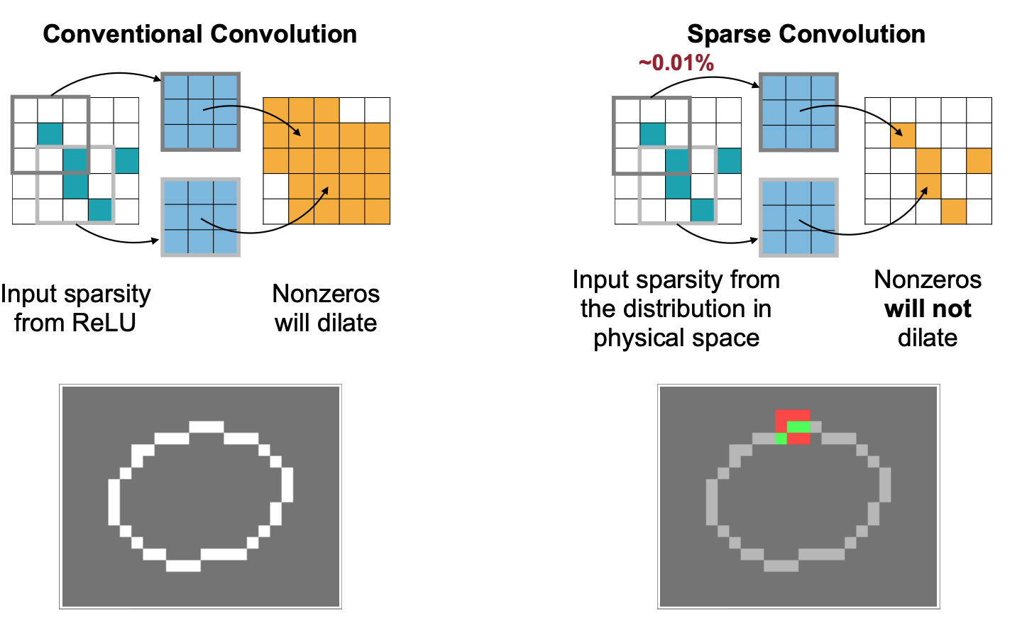
Sparse Convolution은 Point cloud 환경에서 아래와 같이 들어오는 입력에 Sparsity가 낮을 때 기존에 Convolution이 가지고 있는 연산량의 문제를 해결해주는 Submanifold Sparse Convolutional Neural Networks [Graham, BMVC 2015]에서 나온 내용이다. 아이디어는 입력의 분포를 출력이 동일하게 가져간다는 것으로 이 개념에 대한 자세한 내용은 논문에서 확인하는 걸로.
TorchSparse: Efficient Point Cloud Inference Engine [Tang et al., MLSys 2022]
강의에서는 이 Sparse convolution에서 “zero 파라미터에 대해서 연산을 어떻게 하면 안할 수 있을까?”에 대한 내용이다. 이를 위해 Input, Output, 그리고 Weight의 곱을 Mapping한 Map을 Weight에 대해 정렬한 후, 연산의 결과를 output에 accumulate하는 방식이다. 예를 들어 $Q_4$ 를 중심으로 아래 $W$ 사각형을 그리면 $W_{-1, -1}$과 $W_{1,1}$$P_3$의 곱이 $Q_4$에 누적될 것이다. 이는 반대로 $P_3$ 을 중심으로 커널 $W$ 를 그리고 $W_{-1,-1}$ 과의 곱이 원점을 기준으로 대칭인 출력값에 누적된다고 생각할 수도 있을 것이다(그게 바로 위에 그림!).

TorchSparse: Efficient Point Cloud Inference Engine [Tang et al., MLSys 2022]
이렇게 Sparse Convolution 연산에서 최적화는 앞서 Input $P$ 와 Output $Q$의 연산에서 Kernel $W$와 Mapping이 될텐데, 이를 $W$ 를 기준으로 정렬을 해서 한번에 계산하는 방식으로 최적화를 한다.
-2.gif)
TorchSparse: Efficient Point Cloud Inference Engine [Tang et al., MLSys 2022]
이를 전체 다이어그램으로 보면 아래와 같다. Input F에 Locality-Aware: Gather 의 경우 Weight에 해당하는 Input F를 모으는 단계일 테고, Output F의 경우는 각 Weight와 Input F의 곱으로 계산한 결과를 Output F에 Accumulate 하는 단계가 Locality-Aware: Scatter Accumulate 일 것이다.

TorchSparse: Efficient Point Cloud Inference Engine [Tang et al., MLSys 2022]
앞선 방법은 우리는 연산의 redundancy를 줄이려 한다. 그러면 redundancy를 줄인 상태에서 연산을 더 빠르게 할 수 있는 방법으로 P unit의 연산을 어떻게 Parellel하게 진행시킬 수 있을까? 에 대한 방법이 바로 “Regularity”를 만드는 것이다. 두번째 Regularity는 예제중 나온 Load balancing과 유사한 개념이다. overhead를 잡고 regularity를 높인다는 말인데, 가능한 비슷한 크기의 Matrix끼리 묶는 아래 그림에서 마지막 케이스와 같은 방식이다.

TorchSparse: Efficient Point Cloud Inference Engine [Tang et al., MLSys 2022]
마지막은 PointAcc: Efficient Point Cloud Accelerator 에서 Input $P$ 과 Kernel $W$ 연산에서 Output $Q$와의 관계에서 그 연산에 Output에 누적하는 관계가 원점대칭으로 Kernel의 중심으로 부터 연산하는 Weight의 위치 만큼 평행이동하는 지점의 Output에 연산되는 것을 볼 수 있다. 이를 이용해서 Input Point Cloud의 좌표를 예를 들어 $W_{-1,-1}$ 과 연산할 경우 $+(1,1)$ 씩 위치를 옮긴다음 Input과 Output을 합친 배열을 Merge Sort를 하면, 여기서 Input P 와 Output Q의 위치가 겹치는 경우에 연산을 한다는 것이 이 논문의 아이디어이다.
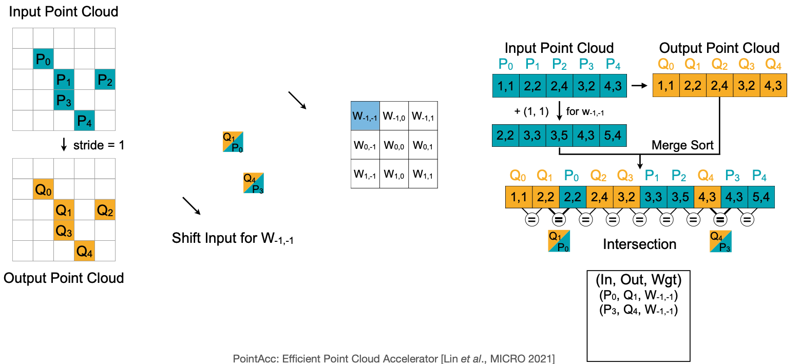
PointAcc: Efficient Point Cloud Accelerator [Lin *et al*., MICRO 2021]]
여기까지 Pruning의 정의에서 부터 구체적으로 Pointcloud 라는 분야에 적용할 수 있는 방까지 살펴봤다. 다음 강의에서는 Pruning 다음으로 나오는 Quantization(양자화)에 대해서 다룰 예정이다.
8. Reference
- EIE: Efficient Inference Engine on Compressed Deep Neural Network
- ESE: Efficient Speech Recognition Engine with Sparse LSTM on FPGA [Han et al., FPGA 2017]
- Sparse GPU Kernels for Deep Learning [Gale et al., SC 2020]
- PatDNN: Achieving Real-Time DNN Execution on Mobile Devices with Pattern-based Weight Pruning [Niu et al., ASPLOS 2020]
- TorchSparse: Efficient Point Cloud Inference Engine [Tang et al., MLSys 2022]
- TorchSparse++ [Tang and Yang et. al, MICRO 2023]
- PointAcc: Efficient Point Cloud Accelerator [Lin et al., MICRO 2021]
- Submanifold Sparse Convolutional Neural Networks [Graham, BMVC 2015]
- MCUNet: Tiny Deep Learning on IoT Devices [Lin et al., NeurIPS 2020]
- On-Device Training Under 256KB Memory [Lin et al., NeurIPS 2022]
- Im2col: Anatomy of a High-Speed Convolution
- In-place Depth-wise Convolution: MobileNetV2: Inverted Residuals and Linear Bottlenecks [Sandler et al., CVPR 2018]
- Winograd Convolution: “Even Faster CNNs: Exploring the New Class of Winograd Algorithms,” a Presentation from Arm
- Winograd Convolution: Fast Algorithms for Convolutional Neural Networks
- Understanding ‘Winograd Fast Convolution’
- TinyML and Efficient Deep Learning Computing on MIT HAN LAB
- Youtube for TinyML and Efficient Deep Learning Computing on MIT HAN LAB