What is p-value ?
\[p = P(\text{Assumption} \lvert \text{ Observation})\ ?\]p-value, “Null hypothesis”
\[\text{p value }=\text{ 1 case + 2 case + 3 case}\]- The probability random chance would result in the observation
- The probability of observing something else tha is equally rare
- The probablity of observing something rarer or more extreme
-
Example for p-value(Two-Sided)
- [Null hypothesis, opposite meaning is “My coin is super special because it landed on Heads twice in a row] In statistic lingo, the hypothesis is even though I got HH in a row, my coin is no different from a normal coin. (H: Head, T: Tail) In this case, the probability is HH 0.25, TT 0.25, HT/TH 0.5. It didn’t matter a order because the first flip didn’t effect the next flip.
- [Null hypothesis] In statistic lingo, the hypothesis is even though I got HHHTH in a row, my coin is no different from a normal coin. (H: Head, T: Tail)
- Probability distribution (refer to the youtube!)
-
One-sided p-value
Linear regression
\[\hat\beta^{LS} = \underset{argmin}{\beta}\{ \displaystyle\sum_{i=1}^n (y_i-x_i\beta)^2 \} = (X^TX)^{-1}X^Ty\] \[\begin{aligned} E(x)&=\displaystyle\sum_{i=1}^Nx_iP(x_i) \\ V(x)&= E((x-m)^2)=\dfrac{1}{N}\displaystyle\sum_{i=1}^N(x_i-m)^2 \\ &= E((x-E(x))^2) = \displaystyle\sum_{i=1}^N P(x_i)(x_i-E(x)) \end{aligned}\] \[\begin{aligned} \text{Expected MSE} &= E[(Y-\hat{Y})^2\lvert X] \\ &= \sigma^2 + (E[\hat Y] -\hat Y)^2 + E[\hat Y -E[\hat Y]]^2 \\ &= \sigma^2 -\text{Bias}^2(\hat Y) + Var(\hat Y) \\ &= \text{Irreducible Error} + \text{Bias}^2 + \text{Variance} \end{aligned}\]$\checkmark$ The goal is removing most of $\beta$, and simplify the linear model!
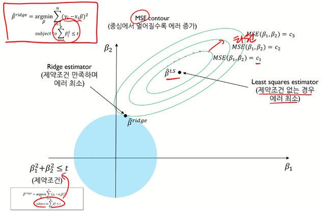
Ridge regression, “L2”
\[\hat\beta^{ridge} = \underset{argmin}{\beta}\{ \displaystyle\sum_{i=1}^n (y_i-x_i\beta)^2 \}, \text{ subject to }\displaystyle\sum_{j=1}^p \beta_j^2 \leq t\]Represent using Lagrange multiplier,
\[\hat\beta^{ridge} = \underset{argmin}{\beta}\{ \displaystyle\sum_{i=1}^n (y_i-x_i\beta)^2 + \lambda \displaystyle\sum_{j=1}^p \beta_j^2 \}\]

Youtube, [핵심 머신러닝] 정규화모델 1(Regularization 개념, Ridge Regression)
$\checkmark$ Cons: Almost $\beta_2$ can be 0, but not 0.
$\checkmark$ Ridge regression is differentiable → closed form solution
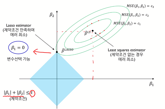
Lasso(Least Absolute Shrinkage and Selection Operator), “L1”
\[\hat\beta^{ridge} = \underset{argmin}{\beta}\{ \displaystyle\sum_{i=1}^n (y_i-x_i\beta)^2 \}, \text{ subject to }\displaystyle\sum_{j=1}^p \beta_j \leq t\] \[\hat\beta^{ridge} = \underset{argmin}{\beta}\{ \displaystyle\sum_{i=1}^n (y_i-x_i\beta)^2 + \lambda \displaystyle\sum_{j=1}^p \beta_j \}\]

Youtube, [핵심 머신러닝] 정규화모델 1(Regularization 개념, Ridge Regression)
$\checkmark$ Cons: $\beta_2$ can be 0, but if data has high covariance, then it lose its robustness
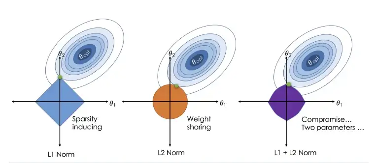
Elastic net, “L1+L2”
\[\hat\beta^{\text{Elastic net}} = \underset{argmin}{\beta}\{ \displaystyle\sum_{i=1}^n (y_i-x_i\beta)^2 + \lambda_1\displaystyle\sum_{j=1}^p \beta_j^2 + \lambda_2\displaystyle\sum_{j=1}^p \beta_j \} \}\]

Figure: An image visualising how ordinary regression compares to the Lasso, the Ridge and the Elastic Net Regressors. Image Citation: Zou, H., & Hastie, T. (2005). Regularization and variable selection via the elastic net.